Hussein M. Badran1, Zaher Khraibani2, Hussein Khraibani2, Hassan Zeineddine2, Aline Mefleh2, Hassan Hamie3
1Islamic University of Lebanon, Faculty of Economics and Business, Beirut, Lebanon
2Lebanese University, Faculty of Sciences, Department of Statistics, Hadath, Lebanon
3Lebanse Petroleum Administration, Beirut, Lebanon
Correspondence to: Zaher Khraibani, Lebanese University, Faculty of Sciences, Department of Statistics, Hadath, Lebanon.
| Email: |  |
Copyright © 2016 Scientific & Academic Publishing. All Rights Reserved.
This work is licensed under the Creative Commons Attribution International License (CC BY).
http://creativecommons.org/licenses/by/4.0/

Abstract
Recently, the East Mediterranean region witnessed frequent extreme climate change conidtions manifested in high waves, strong wind and seismic activity. This resulted in increased attention to the safety of existing oil rigs. Thus, based on the variable dependency of the extreme value theory, the study aims to propose a new method to control the effect of climate conditions, particularly the wind speed, which may inflict structural damage to oil rigs. Additionally, the study seeks to compare the extreme value dependence between two different regions in Lebanon in order to evaluate how oil rigs, which will be installed in Lebanon’s maritime area, resist to high wind speed.
Keywords:
Extremal Dependence, Extreme Values, Oil Rigs, Wind speed, Mediteranea Sea
Cite this paper: Hussein M. Badran, Zaher Khraibani, Hussein Khraibani, Hassan Zeineddine, Aline Mefleh, Hassan Hamie, Dependency Modelling of Natural Rare Phenomena: Application on Oil Rigs, International Journal of Probability and Statistics , Vol. 5 No. 2, 2016, pp. 25-32. doi: 10.5923/j.ijps.20160502.01.
1. Introduction
Millions of barrels of oil equivalent are produced every day. In fact, at the end of 2015 production reached 97 million barrels per day [6]. Geological and geophysical studies conducted in the Lebanese offshore, including the interpretation of 2D and 3D seismic data, have revealed the presence of natural gas resources. Some prospects are located in water areas with a depth of 2,000 meters [11]. The fixed or floating platform shall be designed according to water depth and bathymetry of seabed to resist the extreme weather conditions. The future oil and gas exploration and production activities in the Lebanese offshore shall comply with the Health, Safety and Environment requirements in every phase of the value chain.Nowadays, semi-submersible and dynamically positioned drilling ships are used in exploring and drilling exploratory wells in water depths down to 2,500 meters. The cost to operate these rigs is enormous. Weather-related events can affect drilling operations by causing delays that can incur high costs. For this reason, the univariate extreme value theory has been highlighted in the research literature where the variables are independent and identically distributed [1], [7]. This theory is widely used widely in many disciplines such as hydrology, meteorology, biology, environment, flood, hurricane, finance and insurance [2], [4], [5], [8], [23]. The latest studies have specifically focused on variable dependency [10], [12].In this research paper, the interest is specifically oriented toward the study of the univariate extreme value theory as applied to wind speed, using the classical method of the Block Maxima and the Peak Over Threshold (POT) in order to calculate the return level of significant wind speed over periods of 50, 100, 500 and 1000 years to protect the design of floating semi-submersible. This return level is used by the engineers in the design of oil rigs, and for mooring system to avoid wind risks especially to floating rigs.By using both the Frechet and Weibull distribution respectively in the block Maxima and POT methods, we demonstrate that the POT method is more adequate to study the return levels of the wind speed in Lebanon.Furthermore, we are interested in studying the bivariate extreme value theory to compare the wind speed across two different regions in Lebanon: Jiyeh in Southern Lebanon and Tripoli in Northern Lebanon. The dataset used in this study is composed of daily wind speeds registered every six hours during the period of 9-11-2009 to 10-6-2015. The bivariate extreme value theory studies the dependence between two variables and calculates the extreme conditional quantiles through both the block maxima and POT methods. There are different models in the literature to estimate the parameters of the bivariate extreme distributions [13], [17]. In order to study the dependence of the wind speed in two different regions, we develop three models which are the logistic, asymmetric logistic in the block maxima method and Husler Reiss model in the POT method [15], [16].
2. The Univariate Extreme Value Theory
The classical univariate extreme value theory was developed by Frechet, Fisher and Tippett [3]. Two methods are used for estimating the extreme quantiles [7], [9], [10]. The first one is the block maxima method, which suggests the use of the generalized extreme-value (GEV) to calculate the limit distribution of the maxima or minima based on the Fisher-Tippett theorem [14].Theorem: Let  be a sequence of independent and identically distributed random variables, and
  . If a sequence of pairs of real numbers
  exists such that
  :
:  where
where  is a non degenerate distribution function, then the limit distribution
  belongs to one of the three distributions below called the generalized extreme value
  distributions whose standard forms are:1-Gumbel:
 Where
Where  2-Frechet:
 Where
Where  and
and  is the shape parameter.3-Weibull :
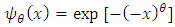 Where
Where  and
and  is the shape parameter.The GEV distribution is given by:
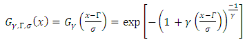 where
where  is such that
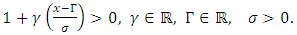
 the location parameter,
  the scale parameter and
  the shape parameter. If
  , we have a Frechet distribution. If
  , we have a Weibull distribution. If
  , we have a Gumbel distribution.The second method is the POT method, which studies the values that exceed a given threshold and uses the Generalized Pareto distribution (GPD) whose survival function is the following:
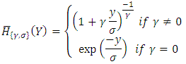 Theorem [13]There is an equivalence between the convergence in distribution of the maximum to a GEV and the convergence in the distribution of the exceedances to a GPD [14]:
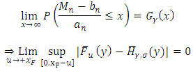 Where
Where  is the endpoint of the function
  .The advantage of the POT method is that it is easier to construct a sample of exceedances than a sample of maxima.Using both methods we can calculate the return level over a period of
  years of a given variable, which is the value of the variable that will be exceeded one time every
  years with a probability of
  .
.
2.1. Block Maxima Method and Parameters Estimation
The classical approach to modelling the extremal properties of an independent and identically distributed variables  is held by using the block maxima method, which relies on probabilistic results based on the Fisher and Tippett (1928) theorem [14]. To apply the block maxima method, we choose to consider a block of 15 days, and thus we have
  observations in each block; therefore, the year is divided into 24 blocks. Finally, we obtain 136 maxima that will constitute the studied sample.The estimation of the GEV distribution parameter is obtained by using the maximum likelihood method [21] with a
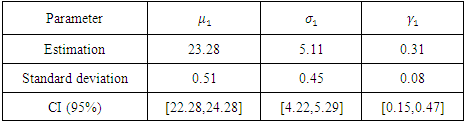
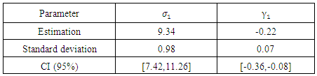
  confidence interval (CI) which is given in the following Table:
Table 1. Estimation of the GEV distribution parameters
 |
| |
|
We find that  , so the distribution of the maximum is a Frechet distribution.To verify this result we use the comparison models method. If we suppose the maxima to be independent and having the same GEV distribution, then for a very high value n, we have the deviance [19]:
 where
where  is the maximum likelihood for the model with
  and
and  the maximum likelihood for the model with
  .So, we condiser the hypothesis
  , we will reject
  if
if  where
where  is the
  quantile with
  .We obtain:
 and
and  Hence,
 The value of D is higher to the critical value
  , so we reject
  and thus
  and the GEV distribution is Frechet.
2.2. Return Level
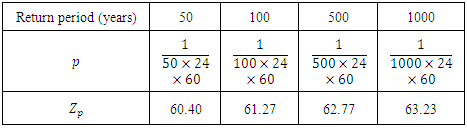
The return levels for the periods of  years are given by the following formulas [19]:
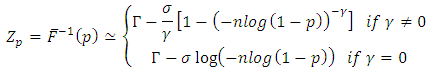 Next we search the value that will be exceeded once every
  observations where
  and
and  the number of observations per block,
  the number of blocks per year. If we consider the value that will be exceeded once every
  blocks then the return level of
  years is:
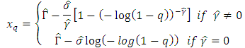 The results obtained by the statistical software (R) are the following [18]:
Table 2. Estimations of the return levels

 |
| |
|
Based on Table 2, the wind speed that will be exceeded once every  blocks is
  , respectively.
2.3. POT Method and Parameters Estimation
To fix a threshold  we consider all the values that exceed it by using the linear mean excess function (MEF), for
  we have [22]:
 With
With  we have:
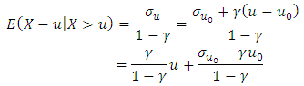 Based on the mean residual life
  plot in the software (R), we choose the value of the wind speed above by which the mean excess function becomes linear.
 | Figure 1. MRL plot |
It seems that above  the MEF becomes linear, so we choose 30 as a threshold and we have 145 exceedances among 8160 observations, which represent
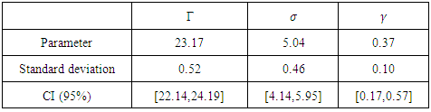
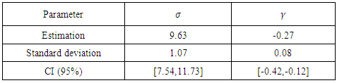
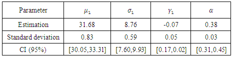
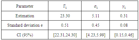
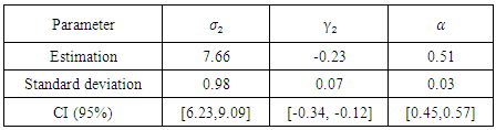
  of the observations.The parameter's estimations are in the following Table:
Table 3. Parameters estimation by GPD
 |
| |
|
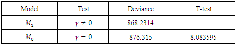
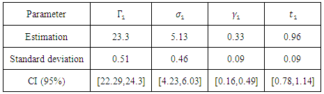
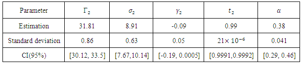
We notice that 0 is not included in the confidence interval.To verify, we consider the below hypothesis: We propose the Analysis of Variance (ANOVA) test:
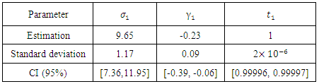
Table 4. Parameter estimations by GPD
 |
| |
|
The statistic test shows that 8.083595 > 3.84 (the  quantile of
  , so we reject
  and hence the corresponding distribution is Weibull.The return level for a period of
  years is given by the following formula [22]:
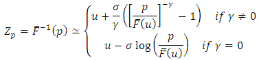 where
where  is the threshold.The obtained results are:
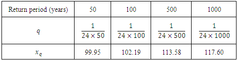
Table 5. Estimation of the return levels
 |
| |
|
Based on Table 5 we can deduce that the wind speed be exceeded once every  and 1440000 observations is 60.40, 61.27, 62.77 and 63.23 km/h, respectively.Finally, by comparing the results of the two methods in the case of univariate extreme values, we notice that there is a considerable difference due to the distributions in both methods being different. In fact, the Frechet distribution gives high and not very realistic return levels for the wind speed unlike the Weibull distribution, which gives more acceptable values.Hence, we can say that the POT method is more appropriate than the block maximum one for the wind speed variable and, thus, the return levels of the wind speed in Jiyeh for periods of 50,100,500 and 1000 years are not very high and risky.
3. Bivariate Extreme Value Theory
The bivariate extreme value theory has so far received little attention in the literature [24]. As the univariate case, the bivariate extreme value is applied in several areas. For example, in the analysis of environmental extreme value data, there is a need of models of dependence between extremes from different sources. We study one more variable, in this section which is the wind speed in Tripoli to test the dependency between it and the wind speed in Jiyeh and then we calculate the conditional probabilities.
3.1. Bivariate Block Maxima Method
The recorded database of the wind speed in Tripoli is similar to that of Jiyeh; we choose the same division of blocks. First we apply the logistic distribution method to estimate the parameters of the bivariate extreme distribution. The bivariate logistic distribution function for a pair of variables
  where each one follows a univariate generalized extreme value distribution is [17]:
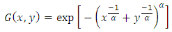 where
where  is the dependence parameter:1. If
  then
then 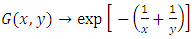 so we have an independence between the two variables.2. If
  then
then 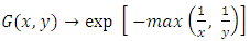 so we have a perfect dependence.The estimated parameters using the maximum likelihood method are in the following Table:
Table 6. Estimation of parameters of case1 of the logistic model
 |
| |
|
Table 7. Estimation of parameters of case 2 of the logistic model
 |
| |
|
 Secondly we apply the bivariate asymmetric logistic distribution function for the pair of variables
  [17]:
[17]: Where
Where  is the dependence parameter,
  and
and  are the asymmetric parameters.1. If
  , we have the logistic model.2. If
  or
or  or
or  , we have an independence.3. If
  and
and  , we have a perfect dependence.The estimated parameters are:
Table 8. Estimation of parameters of case 1 of the asymmetric logistic model
 |
| |
|
Table 9. Estimation of parameters of case 2 of the asymmetric logistic model
 |
| |
|
 Third we apply the bivariate Husler-Reiss distribution function for a pair of variables
  [17]:
[17]: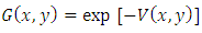 Where
Where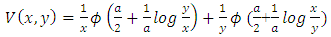 where
where  the normal cumulative distribution
  ; a represents the independence.1. If
  ,
,  i.e we have an independence;2. If
  ,
,  then
then  i.e total dependence.The estimated parameters are:
Table 10. Estimation of parameters of case 1 of Husler-Reiss model
 |
| |
|
Table 11. Estimation of parameters of case 2 of Husler-Reiss model
 |
| |
|
3.2. Models Comparison
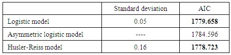
To compare the three previous models and choose the most appropriate one we can use the Akaike information criterion (AIC). The best model is the one with the lowest AIC where 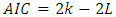 [17].with k: the number of parameters and L: the log likelihood of the model.
Table 12. Models comparison
 |
| |
|
Table 13. Verification of dependence test
 |
| |
|
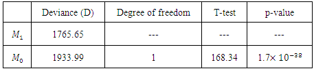
Since the logistic and Husler-Reiss models have the lowest and very similar AIC values, we choose the model with the lowest standard deviation of the dependence parameter, which is the logistic model.To verify the dependence between the two variables, we propose the following statistic test:
 We obtain a p-value < < 5%, so we strongly reject the independence hypothesis
  and thus we conclude the dependency between the two regions in Lebanon.
3.3. Conditional Probability Quantile
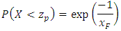
We can also calculate the probability that the wind speed in Jiyeh exceeds a given value given that the wind speed in Tripoli exceeds 50 km/h: We can simplify the calculation by transforming the marginal distribution of
  and
and  into a Frechet distribution. The transformation for Y is the following:
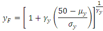 and for
 with the marginal probability of
 and of
 and
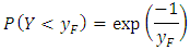
and 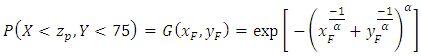 Thereby, we have the graph of the conditional probability:
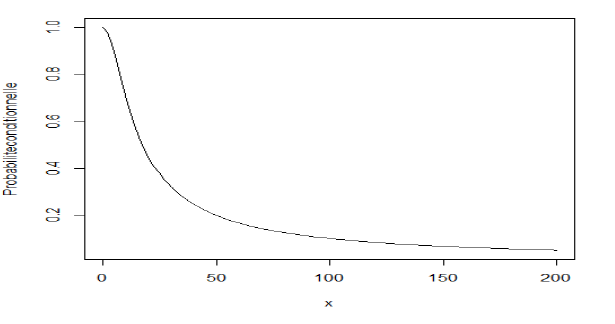 | Figure 2. Conditional probability |
Finally, using this graph, we find that the probability that the wind speed in Jiyeh exceeds 99.95 equal to 
 (return level of 50 years in the univariate case), given that the wind speed in Tripoli is higher than 50 km/h is 0.1.
3.4. Bivariate POT Method
As the univariate case, we choose the threshold for Tripoli wind speed data using the mrl plot [18].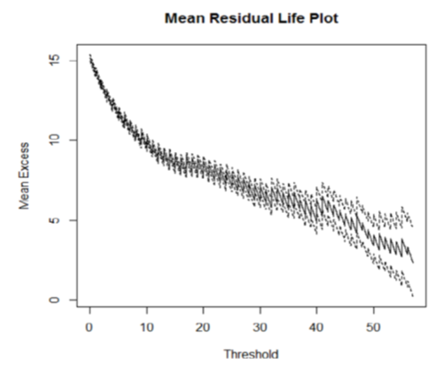 | Figure 3. MRL Plot 2 |
By linearity, we choose  above which there are 138 values that represent 1.69% of the total observations. The parameters are estimated using the censored likelihood method.
 Logistic GPD
Table 14. Estimation of parameters of case 1 of logistic model
 |
| |
|
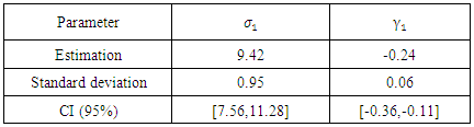
Table 15. Estimation of parameters of case 2 of the logistic model
 |
| |
|
 Asymmetric logistic General Pareto GPD
 Table 16. Estimation of parameters of case 1 of the asymmetric logistic model
 |
| |
|
Table 17. Estimation of parameters of case 2 of the asymmetric logistic model
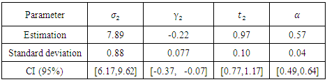 |
| |
|
 Husler-Reiss GPD
 Table 18. Estimation of parameters of case 1 of Husler Reiss model
 |
| |
|
Table 19. Estimation of parameters of case 2 of Husler-Reiss model
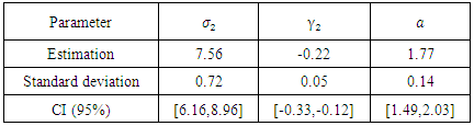 |
| |
|
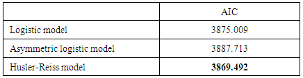
 Models comparison:As before, the best model that will be chosen is the one with the lowest AIC [20].
Table 20. Models comparison
 |
| |
|
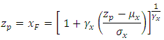
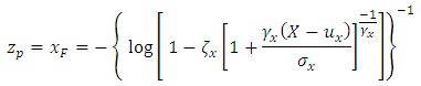
We choose the Husler Reiss model since it has the lowest AIC.To calculate the same conditional probability as before, we transform the marginal distribution of  and
and  into a Frechet distribution.The transformation for
  is:
is: 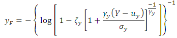 and for
 where
where  and
and  is the number of values that exceed the threshold of the
  variable and n the total number of observations.
 where
where  is the number of values that exceed the threshold of
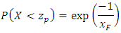
  .So, the marginal probability of
  is:
is: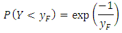 of
of 
 And,
And, where
where  the normal cumulative distribution
  .Finally, the graph of the conditional probability
 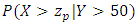 is:
is: | Figure 4. Conidional probability for case 2 |
Using this graph, we find that the probability for the wind speed at Jiyeh to exceed 60.4 km/h (return level of 50 years in the univariate case) given that the wind speed in Tripoli exceeds 50 km/h is 0.68.This probability is high since the added condition is favorable and the difference between the two wind speeds is only 10.4 km/h (60.4-50).
4. Summary and Conclusions
The damage that can be caused by any extreme weather impact on an offshore rig in the future, will surely have huge burden on both the country and the operating companies working offshore Lebanon. The damage is not only limited to financial losses but also to the environmental and social impacts. Results have shown that the return levels of the wind speed in Jiyeh are not very high and risky. The wind speed in Jiyeh and Tripoli dependent on each other and, thus, they almost represent the same risk level since a high value in Tripoli will cause a high value in Jiyeh.The return levels will then be used by engineers to forecast risks and protect the semi-submersible rigs from extreme wind speeds. The problem that remains is the choice of the return level to be used in the design of the rig, this choice will be a trade-off between the desired security level and the cost. So finally, we believe that additional mathematical / statistical analysis should be conducted in future studies. To that end, modeling the return levels related to wave height, can help us evaluate another aspect of the structure integrity for potential offshore rigs.
ACKNOWLEDGMENTS
We would like to acknowledge the Islamic University of Lebanon for the financial support of this research.
References
| [1] | Coles S. (2001). An Introduction to Statistical Modeling of Extreme Values. Springer, London. |
| [2] | Abarbane, H.; Koonin, S.; Levine, H.; MacDonald, G.; Rothaus, O. (January 1992), "Statistics of Extreme Events with Application to Climate" (PDF), JASON, JSR-90-30S, retrieved 2015-03-03. |
| [3] | Haan, L. de and Ferreira, A. (2006). Extreme Value Theory: An Introduction. Springer Series in Operations Research and Financial Engineering, New York. |
| [4] | Embrechts P., Klüppelberg C. and Mikosch T. (1997). Modelling extremal events for insurance and finance. Berlin: Spring Verlag. |
| [5] | Novak S.Y. (2011). Extreme Value Methods with Applications to Finance. Chapman & Hall/CRC Press, London. ISBN 978-1-4398-3574. |
| [6] | Internation Energy Ageny, I. (2015). Oil Market Report. |
| [7] | Lindgren, G.; Rootzen, H. (1987). "Extreme values: Theory and technical applications", Scandinavian Journal of Statistics, Theory and Applications 14: 241–279. |
| [8] | Buishand, T.A., de Haan, L. and Zhou, C. (2008). On spatial extremes: with application to a rainfall problem. Annals of Applied Statistics 2, 624–642. |
| [9] | Smith, R.L. and Weissman, I. (1994), Estimating the extremal index. J.R. Statist. Soc. B 56, 515–128. |
| [10] | Ledford, A.W. and Tawn, J.A. (1997), Statistics for near independence in multivariate extreme values. Biometrika 83, 169– 187. |
| [11] | Hamieh, H. (2015). Lebanese Petroleum Administration. |
| [12] | Tawn, J.A. (1990). Modelling multivariate extreme value distributions. Biometrika 77, 245–253. |
| [13] | Pickands, J (1975). Statistical inference using extreme order statistics, Annals of Statistics 3: 119–131. |
| [14] | Beirlant, J., Goegebeur, Y., Segers, J. and Teugels, J. (2004), Statistics of Extremes: Theory and Appications, Wiley Series in Probability and Statistics, Chichester, U.K. |
| [15] | Lindgren, G.; Rootzen, H. (1987). Extreme values: Theory and technical applications, Scandinavian Journal of Statistics, Theory and Applications 14: 241–279. |
| [16] | J. A. Tawn, Bivariate Extreme Value Theory: Models and Estimation. Oxford. |
| [17] | Ledford, A.W. and Tawn, J.A. (1996). Modelling dependence within joint tail regions, J.R. Statist. Soc. B 59, 475–499. |
| [18] | Coles, S.G.; Heffernan, J. & Tawn, J.A. (1999). Dependence measures for extreme value analyses, Extremes, 2, 339–365. |
| [19] | de Haan, L. & de Ronde, J. (1998). Sea and wind: multivariate extremes at work, Extremes, 1, 7–45. |
| [20] | Falk, M. & Michel, R. (2006). Testing for tail independence in extreme value models, Ann. Inst. Statist. Math., 58, 261–290. |
| [21] | Ledford, A.W. and Tawn, J.A. (1997). Statistics for near independence in multivariate extreme values. Biometrika 83, 169 – 187. |
| [22] | Leadbetter, M. R. (1991). On a basis for 'Peaks over Threshold' modeling, Statistics & Probability Letters 12 (4): 357–362. |
| [23] | Smith, R.L. (2003). Statistics of extremes, with applications in environment, insurance and finance. Chapter 1 of Extreme Values in Finance, Telecommunications and the Environment, edited by B. Finkenst¨adt and H. Rootz´en, Chapman and Hall/CRC Press, London, pp. 1–78. |
| [24] | Ramos, A. and Ledford, A. (2009). A new class of models for bivariate joint tails. J.R. Statist. Soc. B 71, 219–241. |

 Abstract
 Reference
 Full-Text PDF
 Full-text HTML