1. Introduction

The rate of food production in many parts of sub-Saharan Africa has not kept pace with the rate of population growth. Whereas the estimates of population growth rate increase at about 3 per cent annually, that of food production increases by only 2 per cent (Rosegrant et al., 2001). The sub-region's per capita deficit in grains and cereals according to Rosegrant et al., (2001) is one of the highest in the world. Way back in 1967, the sub-region's cereal imports was 1.5 million tons. However, just within thirty years down the way, this figure increased to 12 million tons in 1997, and projections have it that the sub-region will require about 27 million tons of cereal imports to satisfy demand by 2020 (Rosegrant et al., 2001). In the long run, importation may not be economically feasible to ameliorate food shortages. Thus, there is a need to increase domestic production to guarantee food security.

Ghana is still recognized worldwide as an agriculture-based economy. Agriculture has been the anchor of Ghana’s economy throughout post-independence history (McKay and Aryeetey, 2004). While policy and political instability had induced the fall of per capita GDP growth until 1980s, the agricultural sector had been less affected due to less interventions by the government compared to the non-agricultural sector and the fact that its growth is mainly led by smallholder farmers for subsistence purposes. Beyond 1992 when Ghana gained the forth republican political stability, there has been a rapid growth in the nonagricultural sectors; expanding by an average rate of 5.5 percent annually, compared to 5.2 percent for the entire economy (Bogetic et al., 2007).

The analysis presented in this paper suggests that a system of support services; Access to credit facility, Training, Study tour, Demonstrative practical, Networking events and Post-harvest Equipments, plays an important role in determining crop yields even though their individual and interaction effects on yield is not uniform across farmer base organizations. This research focuses primarily on the production of Maize and Soy beans in northern region of Ghana where there exists considerable farming activity. Maize and Soy beans are the very much cultivated in these parts of the country due to their vegetation which supports the growth of grains and cereals. Beyond the numbers and descriptive statistics on yield of such crops, this study tries to bring out variables that significantly contribute to yield. We seek to select among access to credit, training, study tour, demonstrative practicals, networking events, post-harvest equipments, size of plot cultivated and number of farmers; variables (fixed and interaction terms) that significantly influences crop yield in the three Northern regions of Ghana.

2. Variable Selection

Variable selection is aims at choosing the “optimum” subset of predictors. If a model is to be used for prediction, time and/or money can be saved by measuring only necessary predictors. Redundant predictors will add noise to the estimation of other quantities of interest and also lead to loss of some degrees of freedom. Choosing which predictors amongst many potential ones to be included in a model is one of the central challenges in regression analysis. Traditionally, stepwise selection and subset selection are the main means of variable selection for many years. Unfortunately, these methods are unstable and ignores the stochastic errors projected by the selection process.

Many techniques, including ridge regression, least absolute shrinkage and selection operator (LASSO) (Tibshirani 1996), smoothly clipped absolute deviation (SCAD) (Fan and Li 2001), elastic net (EN) (Zou and Hastie 2005), and adaptive lasso (A-LASSO) (Zou 2006) have been projected to select variables and estimate their regression coefficients simultaneously. All these techniques have common advantages over the traditional selection methods; they are computationally simpler, and the derived distributed estimators are stable, and they enhance higher prediction accuracies. These techniques can be cast in the frame of penalized least squares and likelihood. The central benefit of those techniques is that they choose vital variables and estimate their regression coefficients at the same time. In this paper, the H-likelihood (Lee and Oh, 2009) is projected for its special ability to produce penalty functions for variable selection, allow an oracle variable selection and at the same time improve estimation power.

In Agricultural and particularly crop yield analysis, variable selection for decision making in is mostly guided by expert opinion. Very few studies have tried to statistically evaluate these methods in decision making, or to indicate how they might be made better. Variable selection is especially central in the interpretation of Statistical models, particularly, when the actual fundamental model has a distributed representation. Identifying null predictors improves the prediction performances of the fitted model. Notwithstanding, traditional variable selection techniques have two important challenges. First, when the number of predictors is large, it is computationally infeasible to perform subset selection. Secondly, subset selection is extremely unreliable due to its inherent discreteness (Breiman, 1996; Fan and Li, 2001).

To overcome these difficulties, several other penalties have been proposed. The L₂-penalty yields ridge regression estimation, but it does not perform variable selection. With the L₁-penalty, specifically, the penalized least squares (PLS) estimator becomes the least absolute shrinkage and selection operator (LASSO), (Tibshirani, 1996). LASSO is a common method for simultaneous estimation and variable selection, ensuring high prediction accuracy, and enabling the discovery of relevant predictive variables. Donoho and Johnstone (1994) selected significant wavelet bases by thresholding based on an L₁-penalty. Prediction accuracy can sometimes be improved by shrinking (Efron and Morris, 1975) or setting some coefficients to zero by thresholding (Donoho and Johnston, 1994).

LASSO has been criticized on the grounds that a single parameter λ is used for both variable selection and shrinkage. It results in choosing a model with too many variables to forestall over shrinkage of the regression coefficients (Radchenko and James, 2008); otherwise, regression coefficients of the chosen variables are often over shrunken. To surmount this challenge, Fan and Li (2001) proposed a variable selection method based on a non-concave penalized likelihood approach called the smoothly clipped absolute deviation (SCAD) penalty. These methods are distinct from traditional techniques of variable selection in that they remove insignificant variables by estimating their coefficients as 0.

Consequently, their approaches simultaneously select significant variables and estimate regression coefficients. Recent related studies include [Fan and Li 2006, Leng et.al, 2006, Zou and Li, 2008]. More recently, Zou (2006) showed that LASSO does not satisfy Fan and Li’s (2001) oracle property, and proposed the adaptive LASSO. We demonstrate how the h-likelihood methods overcome such difficulties to allow an oracle variable selection and at the same time improve estimation power.

3. Methods

The idea of penalization was initially introduced in the context of solving integral equation numerically by Tikhonov (1943). As is well known, if and K(x, y) is a smooth kernel, the range of the operator with is dense in but not onto. Hence, the inverse A⁻¹ is ill-posed. The solution to the equation

(1)

is difficult to evaluate since approximations to g easily lie beyond R(A). Tikhonov’s solution was to replace (1) by the minimization of

where the Tikhonov’s factor γ > 0 is a regularization parameter and W(f) is a smoothness penalty such as . Numerical (finite dimensional) approximations to this problem are more stable. Note that unless γ = 0, the solution will not satisfy (1).

Generally, regularization is the class of methods required to develop the maximum likelihood to give valid answers in volatile situations. There is a great amount of work in statistics relating to regularization in a broad scope of problems. A thorough survey is beyond the scope of this paper. The central characteristic of most recent data has to do with both size and complexity. The size may allow us to non-parametrically estimate quantities which are ‘unstable’ and ‘discontinuous’ rudimentary functions of the distributions of the data, with the density being a typical instance. Complexity of the data, which usually relates to high dimensionality of observations, makes us attempt more and more complex models to accommodate the data. The fitting of models with a large number of parameters is also inherently unstable (Breiman, 1996). Both of these features, compel us to regularize in order to get sensible procedures. For recent discussions of these issues from different aspects, see Donoho (2000) and Fan and Li (2006). We will consider and relate the LASSO (Tibshirani, 1996), SCAD (Fan and Li, 2001) and H-Likelihood (Lee and Nelder, 2009).

3.1. Least Absolute Shrinkage and Selection Operator (LASSO)

We consider the setting where we have observed data with each a realization of a scalar random variable Y_i, and each a p-vector of explanatory variables. Let X be a matrix with ith row given by . Without loss of generality, we shall require that the columns of X are centred. We assume that

(2)

where each ε_i is i.i.d . In the classical linear model, we would assume X has full column rank, and so p < n. The tuning parameter λ controls the sparsity of the estimate, with large values of λ resulting in estimates with many components set to 0. Unfortunately, this optimization problem is hard, and to the best of our knowledge, it is computationally intractable for p > 50.

The Lasso (Tibshirani, 1996) solves the related problem:

(3)

The non-differentiability of the norm at 0 ensures that the resulting estimator is sparse, and its convexity makes the overall optimization problem convex. There exist very efficient algorithms for solving this problem, even when p > 105 (see for example the R package glmnet).

3.2. The Smoothly Clipped Absolute Deviation (SCAD)

We again analyze the setting where we have (X_i , Y_i), i = 1, … , n, as n observations satisfying

(4)

where Y_i ∈ R is a response variable, X_i is a p_n × 1 covariates vector and ε_i has mean 0 and variance . Here the superscripts are used to make it explicit that both the covariates and parameters may change with n. For simplicity, we assume β₀ = 0. In sparse models. the p_n covariates can be classified into two categories: the important ones whose corresponding coefficients are non-zero and the trivial ones whose coefficients are zero. For notational convenience, we write

(5)

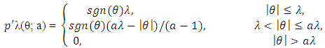
where and . Here is the number of non-trivial covariates. Let be the number of zero coefficients. Let and let be the design matrix. According to the partition of β, write X = ( X₁, X₂), where X₁ and X₂ and and matrices, respectively. Given a > 2 and λ > 0, the SCAD penalty at θ is

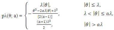(6)

More insight into it can be gained through its first derivative:

(7)

The SCAD penalty is continuously differentiable on (−∞, 0) ∪ (0, ∞), but not differentiable at 0. Its derivative vanishes outside [−aλ, aλ]. Consequently, SCAD penalized regression can produce distributed solutions and unbiased estimates for large coefficients. More in dept analysis of this penalty can be found in Fan and Li (2001). The penalized least squares objective function for estimating β with the SCAD penalty is

(8)

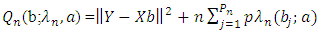
where is the L₂ norm. Given penalty parameters λ_n and a, the LS-SCAD estimator of β is

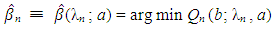(9)

We write the way we partition β into β₁ and β₂.

3.3. Variable Selection Using the Penalized H-Likelihood

In this section, we consider variable selection of fixed effects β by maximizing a penalized profile h-likelihood hp using a weight and a penalty defined by

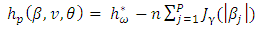(10)

where Jγ (|·|) is a penalty function that controls model complexity using the tuning parameter γ. Normally, setting γ = 0 result in a sub-hazard frailty model, whereas the regression coefficient estimates β approaches 0 as γ → ∞ is inclined to choose a complex model (Fan and Lv, 2010).

Although several penalty functions have been applied in the literature section, (Fan and Li, 2001, 2002; Fan and Lv, 2010), this paper primarily analyze the following three penalty functions.

• LASSO (Tibshirani, 1996)

(11)

• SCAD (Fan and Li, 2001)

(12)

where a = 3.7 and denotes the positive part of x, i.e. is x if x > 0, zero otherwise.

• HL (Lee and Oh, 2009)

(13)

where

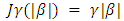
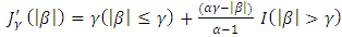
An acceptable penalty function should provide estimates that satisfy unbiasedness, sparcity, and continuity (Fan and Li, 2001, 2002). The LASSO penalty in (11) is as general as L₁ penalty, but it does not satisfy these three properties at the same time. Fan and Li (2001) proved that SCAD in (12) meet all the three properties and that it can perform the orcale process in terms of choosing the correct subset model and estimating the true non-zero coefficient, at the same time.

Lee and Oh (2009) proposed a new penalty unbounded at the origin in the structure of a random effect model. The form of the penalty changes from a quadratic shape (b = 0) for ridge regressions to a cusped form (b = 2) for LASSO and then to an unbounded form (b > 2) at the origin. In the case of b = 2, it allows for an uncountable number of gains at zero. The SCAD provides oracle ML estimates (least squares estimators), whereas the HL provides oracle shrinkage estimates. When multi-collinearity exists, shrinkage estimation becomes much better than the ML estimation. Lee et al. (2010, 2011a,b) has shown the importance of the HL approach over LASSO and SCAD methods, with respect to the number of covariates being larger than the sample size (i.e p > n). In reality it has an attribute for a variable selection without losing prediction power. Since in (13) it has a greater sensitivity to alter the penalty than b, we also analyze only a few values for b, e.g. b = 2.1, 3, 10, 30, 50 denoting small, medium and large.

3.4. Penalized H-likelihood Procedure

By maximizing the penalized h-likelihood h_p in (10), we need to analyze the variable and estimate their related regression coefficients at the same time. In other words, those variable whose regression coefficients are estimated as zero are automatically removed. To accomplish this goal, by applying h_p, the estimation process of the fixed parameters and random effects ν are needed. First, the maximum penalized h-likelihood (MPHL) estimates of (β, ν), are obtained by finding the joint estimating of β and ν:

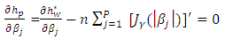(14)

and

(15)

Notice that (14) is an altered estimating equation evoked by adding the penalty term, but (15) is similar to the standard estimating equation without penalty. Notwithstanding, for the three penalty functions considered in (11)-(13), Jγ in (14) becomes non-differentiable at the origin and it does not have continuous second-order derivatives. To elicit this challenge in solving (14) we use local quadratic approximation (referred to as LQA, Fan and Li, 2001) to such penalty functions. That is, given an initial value of β₀ approaching the true value of β, the penalty function Jγ can be locally approximated by a quadratic function as

(16)

Then the negative Hessian matrix of β and ν founded on h_p can be explicitly written as a simple matrix from (Ha and Lee, 2003):

(17)

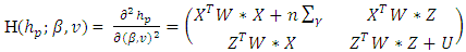
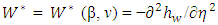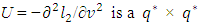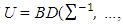
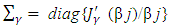
Where . Here X and Z are n × q and n × q∗ model matrices for β and v whose ijth row vectors are and respectively, is a form of the symmetric matrix given in Appendix 2 of Ha and Lee (2003) and Ha et al. (2013) η = Xβ + Zν and matrix that takes a form of if , where and BD(·) represents a block diagonal matrix.

Following Ha and Lee (2003) and (15), it can be observed that given θ, the MPHIL estimates of (β, ν) are obtained from the following scores equations:

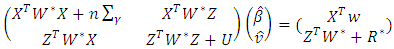(18)

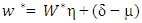
where with and . Here w is the weight w_ij and is the baseline cumulative sub-hazard function. The scores of equations (16) are extensions of the already existing estimation processes. For instance, under no penalty (i.e. γ) they become the score equations of Ha et al. (2003) for the standard sub-hazard frailty models, for variable selection under the Fine-Gray model (1999) without frailty. They also change to

(19)

suggesting that the new equations (16) allow a special case of the penalized equation (17) for the Fine-Gray model. Observe that, to refrain from some numerical complications, we apply , in solving (16) for a small non-negative value of , rather than , to assert the existence of (Lee and Oh, 2009). So far as is small non-negative value, the diagonal component of are similar to that of . As a matter of fact, this algorithm is similar to that of Hunter and Li (2005) for modifying the LQA; see also Johnson et al. (2008). In this paper, we report if all five printed decimals are zero. In the case of, SCAD and HL penalties, there exist many local maximums. Hence, an acceptable initial value is vital to get a proper estimate . In this paper, a LASSO solution will be applied as the initial value for the SCAD and HL penalties.

Consequently, we apply an adjusted profile h-likelihood p_τ (h_p) for the estimation of θ (Ha and Lee, 2003; Lee et al., 2006) which removes (β, v) from h_p in (11), defined by

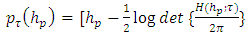(20)

where and . By solving the score equations ∂p_τ(hp)/∂θ = 0 as in Ha et al. (2013), the estimates of θ are found. Consequently, we observe that the projected process is easily implemented by a little change to the already existing h-likelihood process (Ha and Lee, 2003; Ha et al., 2011, 2013).

4. Results

4.1. Simulation Analysis

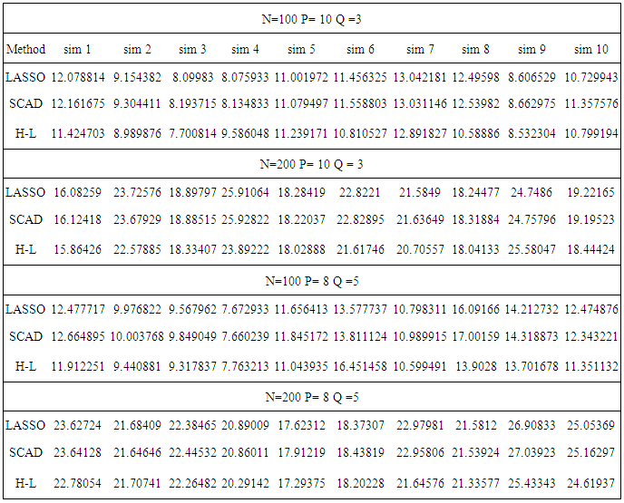
In this section, the performance of the HL method is examined through simulated data, and compared to the LASSO and SCAD. For each method we select optimal tuning parameters that maximize the log-likelihood obtained from an independent validation dataset of size n /2, where n is the size of the training set. We varied the number of covariates (p) and fixed coefficients (q) in two simulations. In one simulation we use n = 200 while in the other n = 100.

For the simulation studies, we consider the following GLM:

with linear link function where the linear predictor consist of p covariates. To generate covariate , we first generate random variables independently from the standard normal distribution. Then are simulated with a multivariate normal distribution. The covariate are generated from

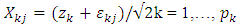(21)

where with covariance structure and ε_kj ∼ N(0, I_p) that of independent of z. The true non-zero coefficients are

β_kj = c/ j, j = 1, . . . , q_k, k ≠ A

where q_k is the number of non-zero coefficients in the kth group, and A is the set of the non-null groups.

A group is said to be non-null if at least one coefficient in the group is estimated to be non-zero. The constant c is chosen so that the signal-to-noise ratio is equal to 5 in the linear model. For each model setting we consider one dimensionality level only, the one with p < n. So, overall we have 4 simulation scenarios, where each is replicated 100 times with sample size n = 200 and n = 100. The cross validation errors which are defined based on independent test sample of size N = 5000 forms the basis for performance comparison. For variable selection quality, cross validation errors for the three methods are compared and the method with the smallest penalized cross validation errors is preferred. The results are shown in table below. The HL estimator performs better than the other methods for prediction accuracy as evident by its smallest cv errors comparative to the other methods.

Table 1. Comparative simulation results for penalized variable selection methods

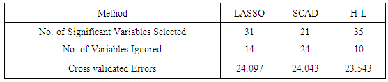
4.2. Real Data Analysis (Crop yield data)

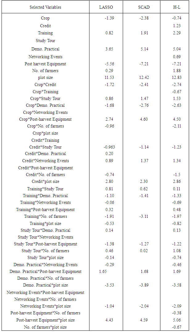
We analyze the crop yield datasets obtained from 2013 main season yield measured in kilograms. The data consists of a numeric response variable (yield) and 9 covariates obtained from 790 farmer based organizations in the three northern regions of Ghana. We excluded 10 observations (FBO’s) due to missing values. The dataset has 7 categorical covariates crop type (Maize or Soybean), Financial Credit (Acquired or Not), Training (Acquired or Not), Study tour (Acquired or Not), Demonstrative Practical (Acquired or Not), Networking Events (Acquired or Not), Post-harvest Equipment (Acquired or Not)) and 2 continuous variables, including plot size in acres and number of farmers. Beside these 9 fixed effects, 36 two-way interaction terms are also generated as fixed interaction terms. This brings the total number of fixed covariates to 45. To allow possible non-linear effects, a third-degree polynomial is used for each continuous covariate, and dummy variables are used for categorical variables.

The results are obtained by 100 random segments of the data set divide into training (70 percent) and test sets (30 percent). For each random segment, the tuning parameters are chosen by the 10-fold cross validation in the training set, and the prediction errors are calculated on the test set. Table 3 presents averages of cv errors, the number of significant variables and number of insignificant variables.

The HL estimator performs better than the other methods for prediction accuracy as evident by its smallest cv errors comparative to the other methods.

Table 2. Standardized Penalized Coefficients of Crop Yield Data

Table 3. Performance of Penalized methods on Crop Yield Data

5. Discussion

In section 4.2, we sort to select significant variables amongst a number of latent ones to be included in the model through penalized methods. We have compare the sparsity and number of significant crop yield variables selected by the three penalized methods; LASSO, SCAD, and H-likelihood both through simulation studies and by the real data (See Table 1 and 2). These techniques have common benefits over the classical selection procedures; they are computationally easy, deriving sparse estimators that are stable, and they aid higher prediction accuracies. We have shown how to choose significant variables amongst common semi-parametric models via penalized methods. We have also shown through numerical studies and data analysis that the projected process with H-Likelihood performs best followed by SCAD, with LASSO coming last (See Table 1 and Table 3).

There has been a number of criticisms against LASSO with some reasons being that a single tuning parameter is utilized for variable selection and shrinkage. A model with too many variables is usually chosen to prevent over shrinkage of the regression coefficients (Radchenko and James, 2008); otherwise, regression coefficients of selected variables are often over-shrunken. This assertion is highly confirmed by the results of this in table 1.

To overcome this problem, a method known as the smoothly clipped absolute deviation (SCAD) penalty for oracle variable selection was proposed by Fan and Li (2001). More recently, Zou (2006) showed that LASSO does not satisfy Fan and Li’s (2001) oracle property, and proposed the adaptive LASSO. Based on the findings of this study, we also propose the H-likelihood approach by Lee and Nelder (2009), as the best in crop yield variable selection and we do so on the basis that, compared to other forms of penalized methods ie. LASSO and SCAD, the H-likelihood approach (Lee and Nelder 2009) facilitates higher prediction accuracy since it has least estimated penalized cross validated errors (see table 2).

6. Conclusions

H-Likelihood method of penalized variable selection performs best followed by SCAD, with LASSO coming last. It does both selection of significant variables and estimation of their coefficients simultaneously with the least penalize cross-validated errors compared to the SCAD and the LASSO. We recommend that a deliberate effort be put into strengthening the Agricultural support systems as a form of strategy for increasing crop production in Northern Ghana. Access to credit, training, access to post harvest equipments, access to demonstrative practicals and access to large plot size are the physical support services highly recommended by this study.