-
Paper Information
- Paper Submission
-
Journal Information
- About This Journal
- Editorial Board
- Current Issue
- Archive
- Author Guidelines
- Contact Us
International Journal of Probability and Statistics
p-ISSN: 2168-4871 e-ISSN: 2168-4863
2015; 4(2): 51-64
doi:10.5923/j.ijps.20150402.03
Bayesian Estimation and Inference for the Generalized Partial Linear Model
 Abstract
 Reference
 Full-Text PDF
 Full-text HTML
Haitham M. Yousof1, Ahmed M. Gad2
1Department of Statistics, Mathematics and Insurance, Benha University, Egypt
2Department of Statistics, Cairo University, Egypt
Correspondence to: Ahmed M. Gad, Department of Statistics, Cairo University, Egypt.
| Email: |  |
Copyright © 2015 Scientific & Academic Publishing. All Rights Reserved.
In this article we propose a Bayesian regression model called the Bayesian generalized partial linear model which extends the generalized partial linear model. We consider Bayesian estimation and inference of parameters for the generalized partial linear model (GPLM) using some multivariate conjugate prior distributions under the square error loss function. We propose an algorithm for estimating the GPLM parameters using Bayesian theorem in more detail. Finally, comparisons are made between the GPLM estimators using Bayesian approach and the classical approach via a simulation study.
Keywords: Generalized Partial Linear Model, Profile Likelihood Method, Generalized Speckman Method, Back-Fitting Method, Bayesian Estimation
Cite this paper: Haitham M. Yousof, Ahmed M. Gad, Bayesian Estimation and Inference for the Generalized Partial Linear Model, International Journal of Probability and Statistics , Vol. 4 No. 2, 2015, pp. 51-64. doi: 10.5923/j.ijps.20150402.03.
Article Outline
1. Introduction
- The semi-parametric regression models are intermediate step between the fully parametric and nonparametric models. Many definitions of semi-parametric models are available in literature. The definition that will be adopted in this article is that the model is a semi-parametric model if it contains a nonparametric component in addition to a parametric component and they need to be estimated. The semi-parametric models are characterized by a finite-dimensional component,
 and an infinite-dimensional
  Semi-parametric models try to combine the flexibility of a nonparametric model with the advantages of a parametric model. A fully nonparametric model will be more robust than semi-parametric and parametric models since it does not suffer from the risk of misspecification. On the other hand, nonparametric estimators suffer from low convergence rates, which deteriorate when considering higher order derivatives and multidimensional random variables. In contrast, the parametric model carries a risk of misspecification but if it is correctly specified it will normally enjoy
  with no deterioration caused by derivatives and multivariate data. The basic idea of a semi-parametric model is to take the best of both models. The semi parametric generalized linear model known as the generalized partial linear model (GPLM) is one of the semi-parametric regression models, See Powell (1994); Rupport et al. (2003); and Sperlich et al. (2006).Many authors have tried to introduce new algorithms for estimating the semi-parametric regression models. Meyer et al. (2011) have introduced Bayesian estimation and inference for generalized partial linear models using shape-restricted splines. Zhang et al. (2014) have studied estimation and variable selection in partial linear single index models with error-prone linear covariates. Guo et al. (2015) have studied the empirical likelihood for single index model with missing covariates at random. Bouaziz et al. (2015) have studied semi-parametric inference for the recurrent events process by means of a single-index model.The curse of dimensionality problem (COD) associated with nonparametric density and conditional mean function makes the nonparametric methods impractical in applications with many regressors and modest size samples. This problem limits the ability to examine data in a very flexible way for higher dimensional problems. As a result, the need for other methods became important. It is shown that semi parametric regression models can be of substantial value in solution of such complex problems. Bayesian methods provide a joint posterior distribution for the parameters and hence allow for inference through various sampling methods. A number of methods for Bayesian monotone regression have been developed. Ramgopal et al (1993) introduced a Bayesian monotone regression approach using Dirichlet process priors. Perron and Mengersen (2001) proposed a mixture of triangular distributions where the dimension is estimated as part of the Bayesian analysis. Both Holmes and Heard (2003) and Wang (2008) model functions where the knot locations are free parameters with the former using a piecewise constant model and the latter imposing the monotone shape restriction using cubic splines and second-order cone programming with a truncated normal prior. Johnson (2007) estimates item response functions with free-knot regression splines restricted to be monotone by requiring spline coefficients to monotonically increasing. Neelon and Dunson (2004) proposed a piecewise linear model where the monotonicity is enforced via prior distributions; their model allows for flat spots in the regression function by using a prior that is a mixture of a continuous distribution and point mass at the origin. Bornkamp and Ickstadt (2009) applied their Bayesian monotonic regression model to dose-response curves. Lang and Brezger (2004) introduced Bayesian penalized splines for the additive regression model and Brezger and Steiner (2008) applied the Bayesian penalized splines model to monotone regression by imposing linear inequality constraints via truncated normal priors on the basis function coefficients to ensure monotonicity. Shively et al (2009) proposed two Bayesian approaches to monotone function estimation with one involving piecewise linear approximation and a Wiener process prior and the other involving regression spline estimation and a prior that is a mixture distribution of constrained normal distributions for the regression coefficients.In this article, we propose a new method for estimating the GPLM based on Bayesian theorem using a new algorithm for estimation. The rest of the paper is organized as follows. In Section 2, we define the Generalized Partial Linear Model (GPLM). In Section 3, we present the Bayesian estimation and inference for the (GPLM). In Section 4, we provide Simulation Study. Finally, some concluding remarks and discussion are presented in Section 5.
2. Generalized Partial Linear Model (GPLM)
- The GPLM model has the form
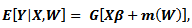 | (1) |
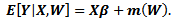 | (2) |
 can be found for known
  and an estimator
  can be found for known
  The estimation methods that will be considered are based on kernel smoothing methods in the estimation of the nonparametric component of the model, therefore the following estimation methods are presented in sequel.
2.1. Profile Likelihood Method
- The profile likelihood method introduced by Severini and Wong (1992). It is based on assuming a parametric model for the conditional distribution of Y given X and W. The idea of this method is as follows:First: Assume the parametric component of the model, i.e., the parameters vector,
 Second: Estimate the nonparametric component of the model which depends on this fixed
  i.e.
i.e.  by some type of smoothing method to obtain the estimator
  Third: Use the estimator
  to construct profile likelihood for the parametric component using either a true likelihood or quasi-likelihood function. Fourth: The profile likelihood function is then used to obtain an estimator of the parametric component of the model using a maximum likelihood method.Thus the profile likelihood method aims to separate the estimation problem into two parts, the parametric part which is estimated by a parametric method and the nonparametric part which is estimated by a nonparametric method.Murphy and Vaart (2000) showed that the full likelihood method fails in semi-parametric models. In semi parametric models the observed information, if it exits, would be an infinite-dimensional operator. They used profile likelihood rather than a full likelihood to overcome the problem, the algorithm for profile likelihood method is derived as follows:Derivation of different likelihood functionsFor the parametric component of the model, the objective function is the parametric profile likelihood function which is maximized to obtain an estimator for
  is given by
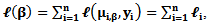 | (3) |
 denotes the log-likelihood or quasi-likelihood function,
 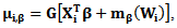 and
and  For the nonparametric component of the model, the objective function is a smoothed or a local likelihood function which is given by
 | (4) |
 and the local weight
  is the kernel weight with
  denoting a multidimensional kernel function and H is a bandwidth matrix. The function in Eq. (4) is maximized to obtain an estimator for the smooth function
  at a point w.Maximization of the likelihood functionsThe maximization of the local likelihood in Eq. (4) requires solving
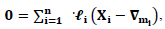
 | (5) |
 Note that
  denotes the first derivative of the likelihood function
  The maximization of the profile likelihood in Eq. (3) requires solving
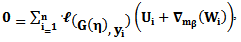 | (6) |
 The vector
  denotes the vector of all partial derivatives of
  with respect to
  A further differentiation of Eq. (5) with respect to p leads to an explicit expression for
  as follows:
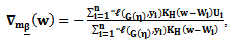 | (7) |
 denotes the second derivative of
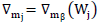
  Equations (5) and (6) can only be solved iteratively. Severini and Saitniswalis (1994) presented a Newton-Raphson type algorithm for this problem as follows:Let
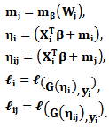 Further let
  and
and  will be the first and second derivatives of
  and
and  with respect to their first argument. All values will be calculated at the observations
  instead of the free parameter w. Then Equations (5) and (6) are transformed to
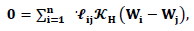 | (8) |
 | (9) |
 based on Eq. (7) is necessary to estimate
 | (10) |
 and
and  obtained from fitting a parametric generalized linear model (GLM).• Using
  and
and 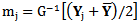 with the adjustment for Binomial responses as
 • Using
  and
and  with the adjustment for binomial responses as
 . (See Severini and Staniswalis, 1994).Second: The updating step for
 where B is a Hessian type matrix defined as
 and
and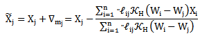
 The updating step for p can be summarized in a closed matrix form as follows:
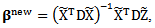 where
where
 The matrix X is the design matrix with rows
  I is an
  identity matrix,
 | (11) |
 | (12) |
 is a smoother matrix with elements
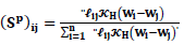 | (13) |
 The function
  is updated by
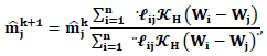 where k=0, l, 2,…is the number of iteration.It is noted that the function
  can be replaced by its expectation with respect to Y to obtain a Fisher scoring type algorithm (Severini and Staniswalis, 1994).The previous procedure can be summarized as follows.Updating step for
 Updating step for
 Notes on the procedure:1. The variable
  which is defined here, is a set of adjusted dependent variable.2. The parameter
  is updated by a parametric method with a nonparametrically modified design matrix
  3. The function
  can be replaced by its expectation, with respect to y, to obtain a Fisher scoring type procedure.4. The updating step for
  is of quite complex structure and can be simplified in some models for identity and exponential link functions G.
2.2. Generalized Speckman Method
- Generalized Speckman estimation method back to Speckman (1988). In the case of identity link function G and normally distributed Y, the generalized Speckman and profile likelihood methods coincides with no updating steps are needed for the estimation of both
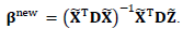
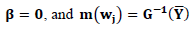
 and m. This method can be summarized in the case of identity link (PLM) as follows:(1) Estimate p by:
 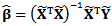 (2) Estimate m by:
  where
where and a smoother matrix S is defined by its elements as
  This matrix is a simpler form of a smoother matrix, and differs from the one used in Eq. (13) where the matrix S yields
  and
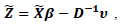
and  in the case of normally distributed Y.For the GPLM, the Speckman estimator is combined with the IWLS method used in the estimation of GLM. As it is shown in IWLS each iteration step of GLM was obtained by WLS regression on the adjusted dependent variable. The same procedure will be used in the GPLM by replacing IWLS with a weighted partial linear fit on the adjusted dependent variable given by
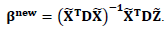
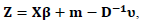 where
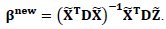
where  and D are defined as in Equations (11) and (12) respectively. The generalized Speckman algorithm for the GPLM can be summarized as: First: Initial values:The initial values used in this method are the same as in the previous profile likelihood algorithm.Second: Updating step for
 Third: Updating step for m
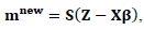 Where
Where
 The smoother matrix is used with elements:
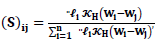 | (14) |
 instead of
  that is used in Equation (14).
2.3. Back-fitting Method
- Hastie and Tibishirani (1990) suggested the back-fitting method as an iterative algorithm to fit an additive model. The idea of this method is to regress the additive components separately on the partial residuals.The back-fitting method will be presented in the case of identity link G (PLM) and non-monotone G (GPLM) as follows:Back-fitting algorithm for the GPLMBack-fitting for the GPLM is an extension to that of PLM. The iterations in this method coincide with that in the Speckman method. This method differs from the Speckman method only in the parametric part. The back-fitting algorithm for the GPLM can be summarized as followsFirst: Initial values:This method often use
 Second: Updating step for
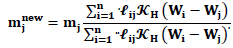
 Third: Updating step for m
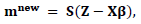 where the matrices D and S, the vector
  are defined as in the Speckman method for the GPLM (See Muller, 2001).In practice, some of the predictor variables are correlated. Therefore, Hastie and Tibshirani (1990) proposed a modified back-fitting method which first search for a parametric solution and only fit the remaining parts non-parametrically.
2.4. Some Statistical Properties of the GPLM Estimators.
- (1) Statistical properties of the parametric component
 Under some regularity conditions the estimator
  has the following properties:1.
  estimator for
  .2. Asymptotically normal.3. Its limiting covariance has a consistent estimator.4. Asymptotically efficient; has asymptotically minimum variance (Severini and Staniswalis (1994).(2) Statistical properties of the non-parametric component m:The non-parametric function m can be estimated (in the univariate case) with the usual univariate rate of convergence. Severini and Staniswalis (1994) showed that the estimator
  is consistent in supremum norm. They showed that the parametric and non-parametric estimators have the following asymptotic properties:
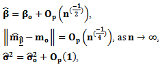 where
where  are the true parameter values so that
3. Bayesian Estimation and Inference for the GPLM
- Bayesian inference derives the posterior distribution as a consequence of two antecedents; a prior probability and a likelihood function derived from a probability model for the data to be observed. In Bayesian inference the posterior probability can be obtained according to Bayes theorem as follows
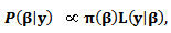 | (15) |
 is the posterior distribution,
  is the prior distribution and
  is the likelihood function.
3.1. A proposed Algorithm for Estimating the GPLM Parameters
- 1. Obtain the probability distribution of response variable,
 2. Obtain the likelihood function of the probability distribution of response variable
  3. Choose a suitable prior distribution of
  .4. Use Eq. (15) to obtain the posterior distribution.5. Obtain the Bayesian estimator under the square error loss function.6. Replace the initial value of
  by the Bayesian estimator.7. Use the profile likelihood method, generalized Speckman method and Back-fitting method with the new initial value of
  to estimate the GPLM parameters.
3.2. Bayesian approach for Estimating the GPLM Using Bayesian Estimator
3.2.1.  is assumed known
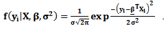
- Case 1Consider the GPLM in Eq. (1) and suppose that
 belongs to the multivariate normal distribution with pdf
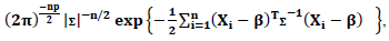
 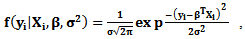 Then the likelihood function of the variable
  can be written as
 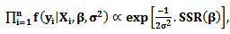 | (16) |
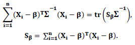
 Let
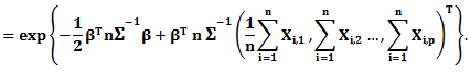
Let Then
Then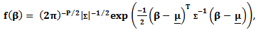 | (17) |
 which is multivariate normal distribution with
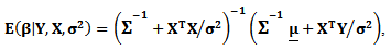
 Then, the Bayesian estimator under the square error loss function
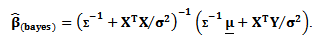 | (18) |
 as follows
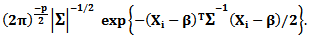 Then the likelihood function of the probability distribution of
  is
is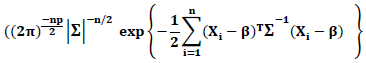
 Let
Let

 Then, we can rewrite the likelihood function of as follows
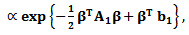 | (19) |
 multivariate normal distribution
  Then
Then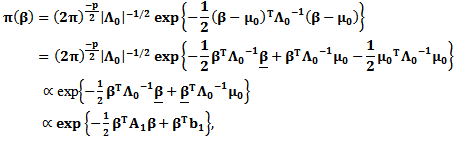 | (20) |
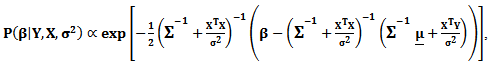
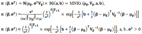
 Combining (19) and (20) and using (15), we obtain the following posterior distribution (using some algebraic steps)
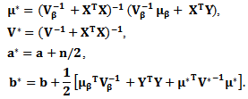
 where
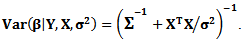
where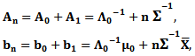 which is multivariate normal distribution with
 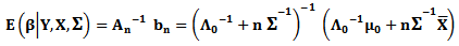 and
and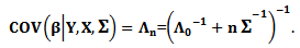 Then, the Bayesian estimator under the square error loss function is
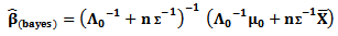 | (21) |
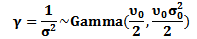
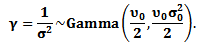
3.2.2.  is assumed unknown
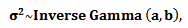
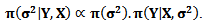
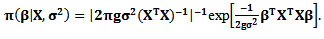
- Case 1 Consider the GPLM in Eq. (1) and suppose that the marginal posterior distribution for
 is proportional with
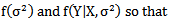
 | (22) |
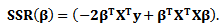
 where
where
 Subsequently
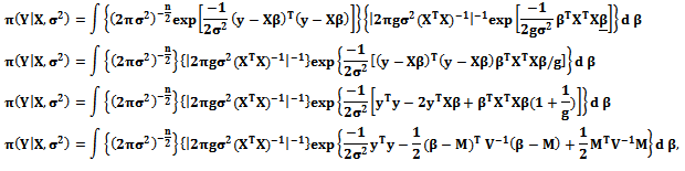 where
where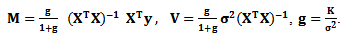
 any positive number, then we can rewrite the last expression as follows
  | (23) |
 Then
Then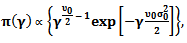 | (24) |
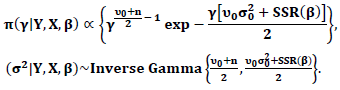
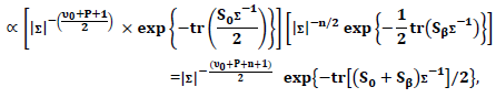
 Therefore
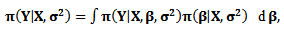
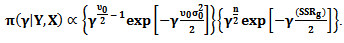
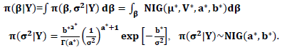
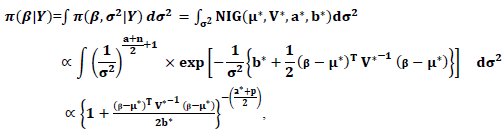
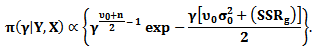 Then, the posterior distribution
 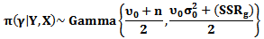 and the marginal posterior distribution for
  is
is 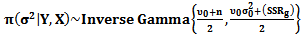 | (25) |
 Then the likelihood function of the pdf of response variable
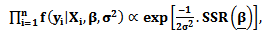 | (26) |
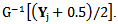
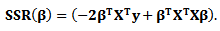
 Let
Let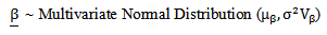 | (27) |
 | (28) |
 | (29) |
 | (30) |
 Then
Then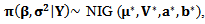 which is normal inverse gamma distribution.From (30), the marginal posterior distribution for
 | (31) |

 | (32) |
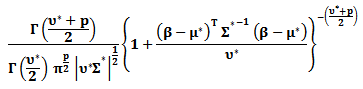 with expected value
  where
where
 Then, the Bayesian estimator under the square error loss function
 | (33) |
3.2.3.  is assumed known
- Case 1Consider the GPLM in Eq. (1) with likelihood function of the pdf of response variable

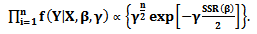 | (34) |
 Then
Then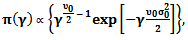 | (35) |
 | (36) |

 | (37) |
 Let
Let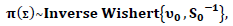 | (38) |
 | (39) |
 with expected value
 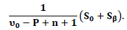 Then, the Bayesian estimator under the square error loss function
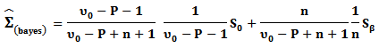 The previous results are summarized in Table (1).
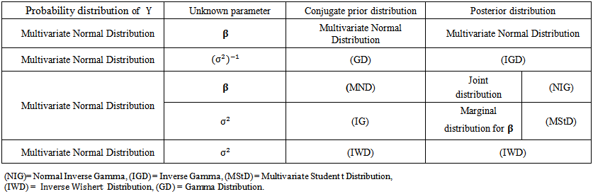 | Table (1). The Posterior Distribution Functions |
4. Simulation Study
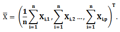
- The aim of this simulation study is twofold. First, is to evaluate the performance of the proposed Bayesian estimators. Second, is to compare the proposed technique with classical approaches. The simulation study is based on 500 Monte Carlo replications. Different sample sizes have been used ranging from small, moderate, to large sizes. In specific sample sizes are fixed at n=50, n=100, n=200, n=500, n=100, and n=2000. Also, different bandwidth parameters are used, namely, h=2, h=1, h=0.5, and h=0.2. The estimation results and statistical analysis are obtained using statistical Package XploRe, 4.8 (XploRe, 2000).The methods are compared according to the following criteria. First, the Average Mean of Squared Errors for
 where
where 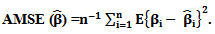 The second is the Average Mean of Squared Errors for
  where
where The third is the deviance where,Deviance = -2 Log Likelihood.The results are shown in the following Tables (2) – (7).
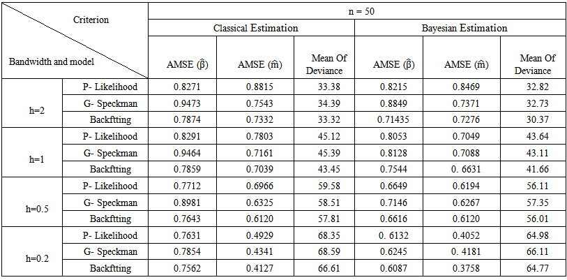 | Table (2). Simulation Results for n = 50 |
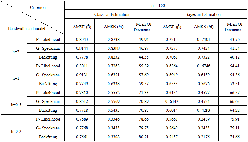 | Table (3). Simulation Results for n = 100 |
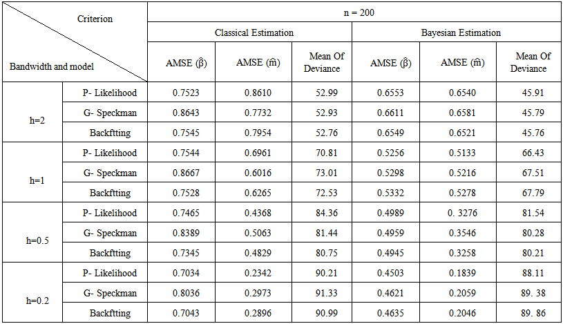 | Table (4). Simulation Results for n = 200 |
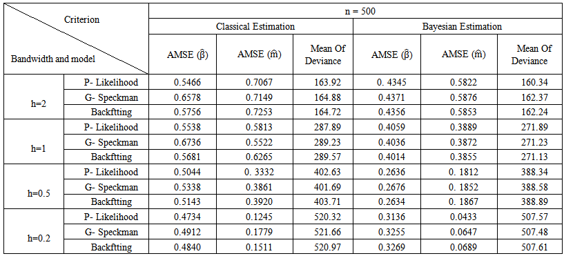 | Table (5). Simulation Results for n = 500 |
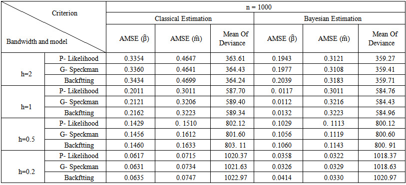 | Table (6). Simulation Results for n = 1000 |
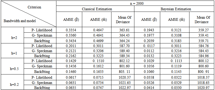 | Table (7). Simulation Results for n = 2000 |
 and Mean of Deviance.2. The Bayesian estimation for the GPLM using the back-fitting method outperforms the profile likelihood method and the generalized Speckman method for n=50 and n=100.3. The Bayesian estimation for GPLM using the profile likelihood method and the generalized Speckman method outperforms the back-fitting method for n=1000 and n=2000.
5. Discussions
- In this article, we introduce a new Bayesian regression model called the Bayesian generalized partial linear model which extends the generalized partial linear model (GPLM). Bayesian estimation and inference of parameters for (GPLM) have been considered using some multivariate conjugate prior distributions under the square error loss function.Simulation study is conducted to evaluate the performance of the proposed Bayesian estimators. Also, the simulation study is used to compare the proposed technique with classical approaches. The simulation study is based on 500 Monte Carlo replications. Different sample sizes have been used ranging from small, moderate, to large sizes. In specific sample sizes are fixed at n=50, n=100, n=200, n=500, n=100, and n=2000. Also, different bandwidth parameters are used, namely, h=2, h=1, h=0.5, and h=0.2. From the results of the simulation study, we can conclude the following. First, the Bayesian estimation for the GPLM outperforms the classical estimation for all sample sizes under the square error loss function. It gives high efficient estimators with smallest AMSE
 AMSE
AMSE  and Mean of Deviance. Second, the Bayesian estimation for the GPLM using the back-fitting method outperforms the profile likelihood method and the generalized Speckman method for n=50 and n=100. The Bayesian estimation for GPLM using the profile likelihood method and the generalized Speckman method outperforms the back-fitting method for n=1000 and n=2000. Finally, The Bayesian estimation of parameters for the GPLM gives small values of AMSE
  AMSE
AMSE  comparable to the classical estimation for all sample sizes.