C. R. Kikawa, M. Y. Shatalov, P. H. Kloppers
Department of Mathematics and Statistics, Tshwane University of Technology, Pretoria, South Africa
Correspondence to: C. R. Kikawa, Department of Mathematics and Statistics, Tshwane University of Technology, Pretoria, South Africa.
| Email: |  |
Copyright © 2015 Scientific & Academic Publishing. All Rights Reserved.
Abstract
Two new approaches (method I and II) for estimating parameters of a univariate normal probability density function are proposed. We evaluate their performance using two simulated normally distributed univariate datasets and their results compared with those obtained from the maximum likelihood (ML) and the method of moments (MM) approaches on the same samples, small n = 24 and large n = 1200 datasets. The proposed methods, I and II have shown to give significantly good results that are comparable to those from the standard methods in a real practical setting. The proposed methods have performed equally well as the ML method on large samples. The major advantage of the proposed methods over the ML method is that they do not require initial approximations for the unknown parameters. We therefore propose that in the practical setting, the proposed methods be used symbiotically with the standard methods to estimate initial approximations at the appropriate step of their algorithms.
Keywords:
Maximum likelihood, Method of moments, Normal distribution, Bootstrap samples
Cite this paper: C. R. Kikawa, M. Y. Shatalov, P. H. Kloppers, Estimation of the Mean and Variance of a Univariate Normal Distribution Using Least-Squares via the Differential and Integral Techniques, International Journal of Probability and Statistics , Vol. 4 No. 2, 2015, pp. 37-41. doi: 10.5923/j.ijps.20150402.01.
1. Introduction
Statistical inference is largely concerned with making logical conclusions about a population using an observed section or part of the entire population referred to as the sample [1]. The reference population can always be represented using an appropriate probability framework which is usually written in terms of unknown parameters. For instance the crop yield obtained when a certain fertilizer is applied can be assumed to follow a normal distribution with mean μ, and standard deviation, σ; it is thereafter required to make inferences about the parameters, μ and σ using the statistics  and
and  that are estimated based on the sample of crop yield and then inferences made on the total crop yield. Note that in this work we only deal with one aspect of statistical inference that is estimation and two novel approaches are discussed in this case.Let x be a single realisation from a univariate normal density function with mean μ, and standard deviation σ, which implies that x~ N(μ, σ) with −∞ < μ < ∞, σ> 0. In this paper, simple and computationally attractive methods for estimating both μ and σ of a univariate normal distributionfunction are proposed. However, methods for estimating the sufficient parameters of a univariate normal density function are well known such as the method of moments and the maximum likelihood method [2, 3], but all these are computationally intensive. Again, much as the maximum likelihood estimators have higher probability of being in the neighbourhood of the parameters to be computed, in some instances the likelihood equations are intractable in the absence of high computing gadgets like computers. Though the method of moments could quickly be computed manually by hand, its estimators are usually far from the required quantities and for small samples the estimates are often times outside the parameter space [4, 5]. In all it is not worthwhile to rely on the estimates from the method of moments.
1.1. Generalized Probability Density Function
When a dataset is presented and critically observed for any characteristics that it may exhibit; statistically called exploratory data analysis, we usually want to study its pattern that can vaguely lead us to a possible probability density function (pdf) that can be taken as its probability frame-work for those data. However, if it requires one to build a whole new frame-work or model, then a lot of work has to be done which is quite demanding. In this section we present a frame-work that nearly suits all the pdfs of continuous random variables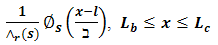 | (1.1) |
where  and
and  indicate the domain of applicability: often times from −∞ to ∞ or from 0 to ∞ depending on the framework under consideration.
  , is the actual shape function of the pdf;
  (the area under the function) is necessary to normalise the integral of the respective function, over the stated to one,
  is the shape parameter,
  and
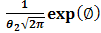
and  are the location and scaleparameters respectively.On examining Eq. (1.1), we present the normal distribution function as
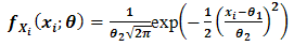 | (1.2) |
Eq. (1.2) represents a normal probability density function with mean  andstandard deviation
  , where
  is a univariate random variable and
  is avector of length, say
  comprising the unknown sufficient parameters [6]. The study presents descriptions and numerical evaluations of two proposed methods intended to estimate the unknown parameters of univariate normal density functions. The proposed methods are compared with two methods in current use, that is the maximum likelihood and method of moments.These are preferred due to their robustness and it is also known that they are symbiotic in that; estimates by the method of moments may be used as the initial approximations to the solutions of the formulated likelihood equations, and successive improved approximations are found using the well-known numerical methods like the Newton-Raphson, Levenberg-Marquardt etc. [7].
2. Method Formulations
It is well known that parameter estimation is an integral part of statistical modelling [8]. In this section we describe two formulations of estimating the univariate normal distribution based on the least-squares method. Linearization of the transcendental model is performed via differentiation and integration methods.
2.1. Theoretical Approach
The main idea is to transform the original problem into a new problem which is linear with respect to a part of the original unknown parameters or their combinations. For instance in the case of the Gaussian density or commonly known as the normal pdf, the transformation is done as in the corresponding system in the following section 2.2. On formulation of a linear system through differential and integral techniques, we finally identify the formulated linear system using ordinary least squares method [9].
2.2. Method I
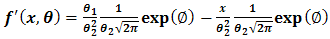
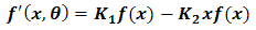
Considering Eq. (1.2) and taking its first derivative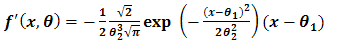 | (2.1) |
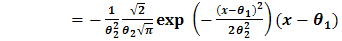 | (2.2) |
From Eq. (2.3), let 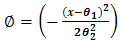 then,
then,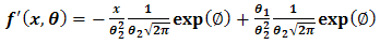 | (2.3) |
 | (2.4) |
Hence Eq (2.4) now becomes,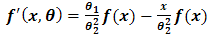 | (2.5) |
 | (2.6) |
where,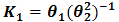 ,
, 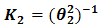 and
and 
 Numerical integral methods [10] are now used to integrate Eq. (2.6) over an interval
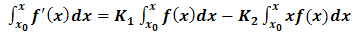 | (2.7) |
 | (2.8) |
where,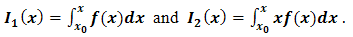 Care should be taken on the numerical procedure for Eq. (2.7) as it is somewhat involved and requires a step by step approach before implementation in any suitable programing language.We now write a complete linear regression function as
 | (2.9) |
Where,  is a regression constant while
  and
and  are the regression coefficients. It has been assume that
  and
and  for the analytical illustration otherwise these could be included in Eq. (2.9). However, in real practise this assumption could be violated without compromising the accuracy of the method. There are a variety of methods for solving linear regression models of the form presented in Eq. (2.9), such as Gauss-elimination, QR-decomposition, least-squares and total least-squares [11]. In this work, the ordinary least-squares (OLS) method is preferred for its simplicity and it is applied to estimate the parameter coefficients
  and
and  . The OLS method is well known and available in a number of statistical literature, for the estimation procedure using OLS the reader is referred to [9]. The parameters of the univariate normal density function can then be computed by applying straight forward algebra, hence
 and
and
 Using an appropriate univariate dataset, the computed estimates can now be compared with those from the method of moments and maximum likelihood methods, and standard statistical measures applied to ascertain the accuracy of the proposed method.
2.3. Method II
The main difference between this method and that formulated in the preceding section 2.3, is that numerical integration techniques were applied on Eq.(2.8). However, for the current method II, the well-known method of integration by parts [12] is applied at the same stage, to obtain,
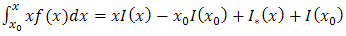 | (2.10) |
where, From method I, Eq. (2.7) can now be written as
 | (2.11) |
 | (2.12) |
Where, . Note, that numerical integration is required at appropriate steps for this second method as well. Eq. (2.13) is then estimated using standard OLS method [9] and the required parameters estimated as
 and
and
 The main difference between these two approaches is that, in method I, we considered use of numerical integration at an earlier step, Eq. (2.7), but in method II, the conventional method of integration by parts is considered and numerical integration on Eq. (2.12). It is noticed that the application of the different approaches of integration at the relevant stages causes a significant difference in the accuracy of estimates from the two estimation methods. Two Monte Carlo numerical simulations are performed using Mathematica software. Mathematica provides an environment in which programming of the proposed approaches is performed and application of the maximum likelihood and the method of moments on the simulated datasets.
3. Simulations
To evaluate empirically the performance of the proposed methods, two normally distributed datasets were simulated with known μ and σ. These datasetsare considered to be random samples of some infinite hypothetical population of possible values. It was necessary to consider both the large  and small
  samples as this could probably give a clue on the performance of the proposed methods when applied to samples of varying sizes.It is known that the principal qualifications of acceptable statistics may most readily be seen by their behaviour when derived from large samples [13]. The aim was to ascertain how these different methods reproduced the known parameter estimates (i.e.
  and
and  ) and also provide base of supportto the proposed methods especially when used on large samples. It is stated that “a statistic is said to be a consistent estimate of any parameter, if when calculated from an indefinitely larges ample it tends to be accurately equal to that parameter” [13]. For our work the results from the large sample undoubtedly give a hint on the consistence of the estimates computed from the proposed methods see also Table 6.We have considered the performance of the proposed methods I and II, see sections 2.2 and 2.3, by applying the maximum likelihood (ML) and the method of moments (MM) using two simulated datasets. The small sample
  and the large sample
  methodological evaluations are as presented in the subsequent tables.
4. Results
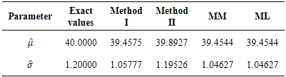
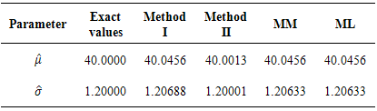
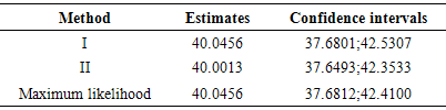
From Tables 1 and 2, we observe that the evaluated methods produce good and acceptable results when compared with the actual or “true” parameters i.e. μ = 40 and  in both large and small samples. However, we haveto understand that these proposed methods cannot be very useful without quantitative statements about their accuracy; in this way it is imperative to evaluate their success. The simplest method of accuracy assessment is based on the confidence intervals of the parameters in question. Confidence intervals can be computed for the accuracy of the point estimate in this case for the mean values presented in Tables 1 and 2. When we require to measure accuracy based on the 95% confidence level, then the interval will be computed as
 where
where  is the estimated mean and
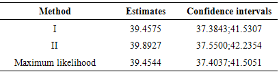
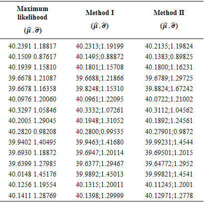
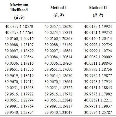
  is the estimated standard deviation. Tables 3 and 4 show the confidence intervals of the estimated mean from both the small and large samples of the estimates computed from methods I and II and the maximum likelihood. It should be noted that we have only considered the estimates from ML method and not MM, since from the latest version of Mathematica (i.e. Mathematica 9), the results from ML and MM are virtually the same in all our computations. In Tables 5 and 6, we presented several results of
  and
and  respectively, computed bybootstrapping from the parent sample or re-sampling. This was aimed at giving a visual analysis on which methods could be better preferred and the sample size on which we could consider using the proposed method for acceptable results.
Table 1. Performance of proposed methods I, II, the maximum likelihood and method of moments, n=24
 |
| |
|
Table 2. Performance of proposed methods I, II, the maximum likelihood and method of moments, n=1200
 |
| |
|
Table 3. The 95% confidence interval of the estimates from the evaluated methods, n=24
 |
| |
|
Table 4. The 95% confidence interval of the estimates from the evaluated methods, n=1200
 |
| |
|
Table 5. Performance of ML, I and II methods on various test bootstrap samples, n=24
 |
| |
|
5. Discussion
From the current work, conventional methods, i.e. maximum likelihood and the method of moments are compared with the proposed methods I and II. The comparison was aimed at visualising how best each of them reproduced the known parameters μ and  . In this case confidenceintervals were computed see Tables 3 and 4 for each of the point estimates (mean value) computed from either methods.The confidence intervals were interpreted to mean that if we had repeated the same sampling scheme a large number of times, we would have expected that in 95% of these experiments the observed accuracy see Tables 1 and 2 for the point estimates; would be somewhere between the respective confidence limits as presented in Tables 3 and 4 in either methods. It should be noted here that we took a risk of 5% that the true means are either less than or greater than the lower and upper boundaries respectively. Therefore, we can narrow the confidence intervals at the expense of committing a greater risk of a Type I error [14]. From Tables 5 and 6, the results of 15 samples of sizes n = 24 and n = 1200 are presented respectively. This was intended to show the performance of either method on both the large and small samples.We cannot over state that, visual inspection is not the best method to ascertain whether or not a given method produces acceptable results and we reserve as future work for an analytical proof that the proposed methods are consistent.
Table 6. Performance of ML, I and II methods on various test bootstrap samples, n=1200
 |
| |
|
6. Conclusions
Considering estimates obtained from the proposed methods and the maximum likelihood, on both the small and large samples, it can be observed that the proposed methods produced relatively acceptable estimates. For the large samples the mean values are the same for all the methods which shows that the proposed methods have the same accuracy as the more trusted and frequently applied maximum likelihood method also regarded as indispensable tool for many statistical modelling techniques [15]. However, the standard deviation estimates differ slightly in each method. The strength of the proposed methods over the maximum likelihood is that the proposed methods do not require starting approximations for the unknown parameters while for the maximum likelihood, it is a requirement for the practitioner to provide starting approximations for the unknown parameters. These starting approximations may not guarantee convergence and may also result in longer computation time if they are far from the required minimum.
ACKNOWLEDGEMENTS
The authors would like to extend their sincere appreciation to the Directorate of Research and Innovation of Tshwane University of Technology for funding this research project under the Postdoctoral Scholarship fund 2014/2015. We also thank the editorial board and the anonymous reviewer who provided insightful comments that led to the improvement of the article.
References
| [1] | Cox, D.R. and D.V. Hinkley, Theoretical Statistics. 1974: Chapman Hall. |
| [2] | Prokhorov, Y.V. and Y.A. Rozanov, Probability Theory, basic concepts. Limit theorems, random processes. 1969: Springer. |
| [3] | Dorfman, D.D. and A.J. Edward, Maximum-likelihood estimation of Parameters of signal-detection theory and determination of confidence intervals rating-method data. Journal of Mathematical Psychology, 1960. 6(3): p. 487-496. |
| [4] | Hall, A.R., Generalized Method of Moments (Advanced Texts in Economics). 2005: Oxford University Press. |
| [5] | Hansen, L.P., Method of Moments in International Encyclopedia of the Social and Behavior Science. 2002, Pergamon: Oxford. |
| [6] | Huber, P.J., Robust Statistics. 1981: Wiley. |
| [7] | NIST, e-Hand book of Statistical Methods. 2003. |
| [8] | Kloppers, P.H., C.R. Kikawa, and M.Y. Shatalov, A new method for least squares identification of parameters of the transcendental equations. International Journal of the Physical Sciences, 2012. 7: p. 5218-5223. |
| [9] | Searle, S.R., Linear Models. 1971: John Wiley and Sons. |
| [10] | Gerald, C.F. and P.O. Wheatley, Applied Numerical Analysis. Third ed. 1983: Addison-Wesley Publishing Company |
| [11] | Elad, M., P. Milanfar, and G.H. Golub. Shap from moments- an estimation theory perspective. in IEE Transactions on Signal Processing. 2004. |
| [12] | Fang, S., Integration by parts for heat measures over loop groups. Journal de Mathematique Pures et Appliques, 1999. 78(9): p. 877-894. |
| [13] | Fisher, R.A. Theory of Statistical estimation. in Mathematical Proceedings of the Cambridge Philosophical Society. 1925. |
| [14] | Rossiter, D.G., Statistical methods for accuracy assesment of classified thematic maps. 2004, International Institute for Geo-information Science and Earth Observation. |
| [15] | Myung, I.J., Tutorial on maximum likelihood estimation. Journal of Mathematical Psychology, 2003. 47(1): p. 90-100. |
 Abstract
 Reference
 Full-Text PDF
 Full-text HTML