1. Introduction

The extreme value theory is a blend of an enormous variety of applications involving natural phenomena such as rainfall, floods, wind gusts, Air pollution, corrosion etc (Chang Hsien-kuo).

Historically, work on extreme value problem may be dated back to as early as 1709 when Nicolas Bernoulli discussed the mean largest distance from the origin when points lie at random on a straight line of length . [see Gumbel, 1958]

In the history of finance, risk management has been identified as one of the most important field of interest to financial and risk Managers in the 20^th century, or rather as among the three major areas of interest following the Markowitz portfolio theory and the Black-Sholes-Merton option pricing theory (Cairns A, 2004). In recent years, we have noticed evidences all over the world the huge development of the field of financial risk management which resulted from the global financial crisis that emerged in 2008 which intensified the need of risk management among financial institutions and insurance companies (TANG Qihe).

The Extreme value theory (EVT) holds promise for advancing assessment and management of extreme financial risks. Recent literature suggests that the application of Extreme value Theory generally results in more precise estimates of extreme quantiles and tail probabilities of financial asset returns (Embrechts P. et al, 1999).

In regard to this paper, the author will discuss concisely the application of Extreme value theory in the field of financial risk management which is the foremost objective for financial institutions and insurance companies by the help of the Random Walk concept.

1.1. Extreme Value Theory

Extreme value theory (EVT) is a tool used to determine probabilities (Risks) associated with extreme events. It is used by Investors in situations where there is/expected to occur higher stress on investment portfolios. The EVT is also used to model the behavior of tips (Maxima) and or dips (Minima) in a series of asset returns etc.

VaR approach was the standard measure of financial risks and other risks such as Industrial risk management etc. Basically, it used to measure the expected loss over a period of time for known distribution of for known probability and under normal market conditions. (Longuin, 1999).

Recently, Portfolio managers, Investors, Risk managers, Claim managers etc, have become more concerned over occurrences under “Extreme market conditions”.

This paper is organized as follows: Section 2 introduces the risk management and approaches to minimize financial risks, section 3 describes the Random walk movement as a result of extremes, and section 4 concluding.

2. Risk Management

Risk management is the process of Identification, Assessment and Decision making over the risks facing an Organization. It can be Formal process which involves Procedures, Quantitative and Qualitative assessments, or it can be Informal (Peter Moles, 2013).

2.1. Approaches for Decision Making

After the risk has been identified on its nature and type, assessment has taken place i.e how big the risk is, the probability to occur and when it is going to happen, then, the decision makers of the Organization or Firm may opt on the following three generic approaches:

• Hedging: Eliminate risk by selling into the market place through cash or spot market transactions or through Forward, Future and Swap contracts.

• Diversification: This reduces risk by combining risks which are not perfectly correlated to form a portfolio.

• Insurance: Risks are transferred from the buyer (Policyholder) to the seller i.e Insurer (Peter Moles, 2013).

3. Intuition of the Random Walk

It is essential for Insurance Companies, Financial Institutions and any profit oriented firm to conduct an evaluation as to when the company is expected to earn a maximum returns or highest profit together with the question how much is that maximum return value.

On the other hand, it would be of important interest for the company to know when it is expected to be ruined so that the required but optimal measures can be adopted against the crisis and also to rescue from loss of potential shareholders and against bad reputation to customers. The company may also be interested to learn whether it will remain liquid forever i.e what happens to the company’s returns at , and ultimately what will be the distribution of the value of so that it can ensure the capital of their shareholders as well as to ensure continuous dividend payments and other benefits to its customers.

This paper tried to explore some mathematical techniques which will be helpful in computing the time at which the company will be at the highest peak (maximum returns) or the least dip (minimum returns), as well as when .

The returns will be mainly expressed in discrete time (Random Walk) and then studying a variety of stopping times using the strong Markov property. The cycles which are generated by stopping times iterates are assumed to be independent and identically distributed.

Let us now introduce the memory less time with distribution where is smaller than (but close to 1 so that is large). Since we are interested with the maximum and minimum before , these will be determined by the last peak stopping time and the last dip stopping time before time respectively.

Now, by distribution

Where and are independent stopping times, similarly

Where denotes the sum of independent random variables, and that and is the value at the highest peak stopping time and the value at the least dip stopping time respectively and they are said to be independent random variables.

3.1. Random Walk

The idea of Radom Walk originated from considering a completely a drunk person who walks with no sense of direction. So she /he may move forward with equal probability that she/he moves backwards. A similar notion is found in financial environment or financial markets where the returns from a single asset have found to be mutually independent and identically distributed.

By definition: If we let be a sequence of independent and identically distributed random variables (Returns), and that to be a stochastic process, then

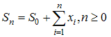Where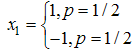

Again let us also consider the following situation

If are independent and identically distributed (i.i.d) random variables and let us fix some set A such that 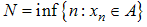i.e the first time any member of to be contained in set A. also we know that

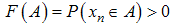Then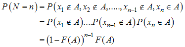

The geometric Random walk model implies that the future is independent of the past and therefore it is not possible to predict the future deviation trends.

3.2. Stopping Times

Stopping time is a random variable which takes place in units of time such that is a function of for all . Examples is like the first time returns of the company reach a certain peak, and or the first time a share price reaches a certain level after dropping by a specified amount.

Let us now consider the iterates of a stopping time such that, if we define be the n-th iterate, and let be defined by , then we can say that

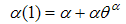Thus, in general

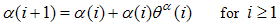In this case a set of independent random stopping times are generated i.e . In other words we can say that for are the peaks such that the returns reaches before falling, and therefore 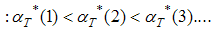in terms of their magnitudes.

But our major interest is on the last peak before time

Let,

Be the counting process associated to the iterates of stopping times , then , for all

Where becomes the last time before memory less time of which we are interested in.

3.3. Random Walk Stopping Times and the Strong Markov Property

A stopping time is a random variable taking values in the time – set including possibly the value of such that is a deterministic function of for all .

The Markov property states that: For any the future process is independent of the past process if we know the present , and thus this remains true if we replace the deterministic by a random stopping time .

Strong Markov property: Suppose is a time – homogeneous Markov chain. Let be a stopping time, then conditional on and , the future process is independent of the past process and has the same law as the original process started from .

3.4. Stopping Times Path into Cycles

Let us also consider another random walk

By tossing a fair coin, let where and , also let us define be the first cycle to contain and that for which

And that are independent and identically distributed random cycles produced by stopping times iterates such that;

3.5. Peaks and Dips of Cycles

In this section therefore, we will concentrate on peaks and dips of various cycles formed during the process, particularly the last peak and dip before success time , that is before the time at which the company attains the maximum value and or the weak minimum value.

Let be the time for the first peak

i.e

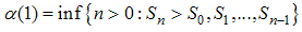it follows that

for and

Similarly,

Let be the time for the first dip

i.e

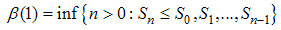and hence

for and

And therefore we can say that is the k-th time value becomes strictly larger than all previous values defined by

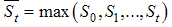Similarly we can also say that is the k-th time takes smaller value than or equal to all previous ones, defined by

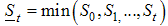Thus, the corresponding counting processes are

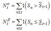For this reason we can say that,

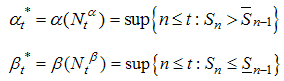Where and are the last peak and dip before hitting time respectively.

Now, from section 1.4, we know that 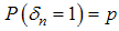and 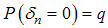; again let us think the situation when and define 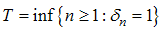then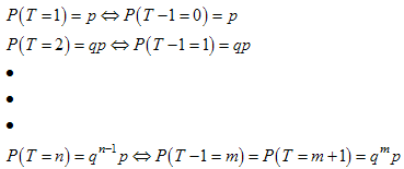

After several observations of tosses of a biased coin, assume now that we got the cycle that contain success.

Let us now define the following notations.

be the last peak before success time

be the last dip before success time

Also, let and be the values of the last peak and dip before success time respectively. And since and they have nothing in common (they are independent), then

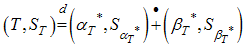
4. Conclusions

The extreme value theory is highly employed in Actuarial industry, particularly in the situations where the Company wants to conduct self performance assessment, identifying investment risks, financial risk assessment, making forecast over a period of time and making any Economical based decisions.

Returns evaluation or financial risk management and time at which the firm is expected to achieve the maximum/minimum returns (profit/loss) are fundamental tasks to the company and to all profit oriented firms (Risk/Claim managers) as this will help them to identify their risk free operating limits in the sense that; it is too risky for the company to operate at extreme points.

For managerial purposes therefore, returns evaluation / assessment has a greater importance to managers and other decision makers to know their risk free operating boundaries.

Lastly, since the computations involve strong mathematical models, we clearly need computer software to be able to reach the targeted goals as it is realy convolution to get solution by hand.