Zoubeida Messali 1, 2, Nabil Chetih 3, Amina Serir 4, Abdelwahab Boudjelal 2
1Department of Electronic, University of El Bachir El Ibrahimi, Bordj Bou Arreridj, Algeria
2Laboratoire de Génie Electrique (LGE), Université de M’Sila, M’Sila, Algérie
3Welding and NDT Research Center (CSC), Cheraga, Algiers, Algeria
4Laboratoire de Traitement d’Images et de Rayonnement (LTIR), Université des Sciences et de la Technologie Houari Boumediene, Alger, Algerie
Correspondence to: Zoubeida Messali , Department of Electronic, University of El Bachir El Ibrahimi, Bordj Bou Arreridj, Algeria.
| Email: |  |
Copyright © 2015 Scientific & Academic Publishing. All Rights Reserved.
Abstract
Images of the inside of the human body can be obtained noninvasively using tomographic acquisition and processing techniques. In particular, these techniques are commonly used to obtain X-ray images of the human body. The reconstructed images are obtained given a set of their projections, acquired using reconstruction techniques. A general overview of analytical and iterative methods of reconstruction in computed tomography (CT) is presented in this paper, with a special focus on Back Projection (BP), Filter Back Projection (FBP), Gradient and Bayesian maximum a posteriori (MAP) algorithms. Projections (parallel beam type) for the image reconstruction are calculated analytically by defining two phantoms: Shepp-Logan phantom head model and the standard medical image of abdomen with coverage angle ranging from 0 to ± 180° with rotational increment of 10°. The original images are grayscale images of size 128 128, 256 256, respectively. The simulated results are compared using quality measurement parameters for various test cases and conclusion is achieved. Through these simulated results, we have demonstrated that the Bayesian (MAP) approach provides the best image quality and appears to be efficient in terms of error reduction.
Keywords:
Computed tomography, Bayesian approach, Reconstruction techniques, Filter Back Projection (FBP), Gradient algorithm
Cite this paper: Zoubeida Messali , Nabil Chetih , Amina Serir , Abdelwahab Boudjelal , A Quantitative Comparative Study of Back Projection, Filtered Back Projection, Gradient and Bayesian Reconstruction Algorithms in Computed Tomography (CT), International Journal of Probability and Statistics , Vol. 4 No. 1, 2015, pp. 12-31. doi: 10.5923/j.ijps.20150401.02.
1. Introduction
During the last decade, there has been an avalanche of publications on different aspects of computed tomography [1-5]. The scientific word tomography means reconstruction from slices. It is an imaging technique which uses the absorption of X-rays by a number of organs in the body. This creates a shadow picture (projection). By sending the X-rays from different angles around the object, a collection of shadow pictures (projections) is created. Combining these pictures results in a tomogram, which is basically the image of a cross-section of the body. The impact of this technique in diagnostic medicine has been revolutionary, since it has enabled doctors to view internal organs with unprecedented precision and safety to the patient. A normal radiography shows mainly the bones and organs within the body. They absorb a major part of the X-rays. The absorption of the X-rays by the neighboring tissue is a lot smaller. This is the reason bones become visible on film, similar to a shadow picture.Given the enormous success of X-ray computed tomography (CT), it is not surprising that in recent years much attention has been focused on extending this image formation technique to nuclear medicine [6] and magnetic resonance on the one hand; and ultrasound and microwaves on the other [7]. In nuclear medicine, our interest is in reconstructing a cross-sectional image of radioactive isotope distributions within the human body; and in imaging with magnetic resonance we wish to reconstruct the magnetic properties of the object. In both these areas, the problem is still the same and can be set up as reconstructing an image from its projections.In tomography, images coming from the computed tomography scan are combined to create a visualization of the scanned body. To create this image we use reconstruction techniques. The most effective type of reconstruction technique is able to reconstruct good quality CT images even when the projected data are noisy. The conventional algorithms of image reconstruction for CT are Back Projection BP and Filtered Back Projection FBP reconstruction techniques which are analytical reconstruction methods. In Filtered Back Projection methodology, Fourier Slice Theorem is made into use for Image reconstruction [8]. Although for now the Filtered Back Projection algorithm is most widely used by manufacturers, efforts have been made to make iterative methods popular again due to their unique advantages, such as their performances with incomplete noisy data. The algebraic reconstruction technique (ART) [1-3], the simultaneous algebraic reconstruction technique (SART) [4] and the simultaneous iterative reconstruction technique (SIRT) [5] are a few of those iterative methods. The algebraic reconstruction technique (ART) [9] was also the first iterative algorithm to be used in CT. ART can be seen as a linear algebraic problem. It is based on the simple assumption that calculating the cross-section can be done by making algebraic equations for the array of unknowns referring to the measured projection data. As well known, simultaneous algebraic reconstruction technique (SART) was proposed as a major refinement of ART, also used in the X-ray tomography, which combines the positive aspect of SIRT and ART. One of the most important iterative reconstruction techniques in CT is the Gradient algorithm [6]. It is considered as an optimization method. More recently, stochastic methods, which are based on the Bayesian framework, have been successfully used in CT [10-13].This article presents the basics of the more widely used algorithms: Back Projection (BP), Filtered Back Projection (FBP), Gradient algorithms and a special focus on a Bayesian maximum a posteriori (MAP) approach. It is not an exhaustive presentation of reconstruction algorithms. Therefore, this paper is aimed to establish a quantitative comparative study of analytical and iterative reconstruction techniques in order to reduce the number of iterations and enhance the image quality. Two Phantoms are used to test the results of the research: the Shepp-Logan Phantom and the standard medical image of abdomen. So, physical phenomena such as attenuation, scattering, and so forth are not under consideration here. The original images are gray scale images of size  respectively.After introducing the basic concepts and the supporting theory in section 2, we present the reconstruction techniques in sections 3 and 4. We focus on developing a Bayesian (MAP) approach, in which the reconstruction is computed by maximizing an associated objective function via an iterative algorithm. Following this, in section 5, we explain how to evaluate the quality of the reconstruction. Section 6 provides some test results and comparisons. Finally, in the last section our conclusions can be read.
2. Basic Formulation
Fundamentally, tomographic imaging deals with reconstructing an image from its projections. In the strict sense of the word, projections are a set of measurements of the integrated values of some parameter of the object-integrations being along straight lines through the object and being referred to as line integrals. A line integral, as the name implies, represents the integral of some parameter of the image along a line as illustrated in Figure 1.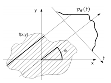 | Figure 1. An object,  and its projection, and its projection,  are shown for an angle of are shown for an angle of  |
The projections (or line integral), as shown in Figure 1, are defined as: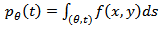 | (1) |
The function  is known as the Radon transform of the function
 , where
  represents the 2D image to be reconstructed, and
  the parameters ofeach line integral.
  is also known as a sinogram of the image. A sinogram as shown in Figure 2, is a 2D image, in which the horizontal axis represents the count location on the detector, and the vertical axis corresponds to the angular position of the detector.
 | Figure 2. (Left) Shepp-Logan phantom head model  (Right) Corresponding sinogram, with coverage angle ranging from 0° to 180 with rotational increment of 10° (Right) Corresponding sinogram, with coverage angle ranging from 0° to 180 with rotational increment of 10° |
Using a delta function,  can be rewritten as:
 | (2) |
It is well known that, from knowledge of the sinogram one can readily reconstruct the image
  by use of computationally efficient and numerically stable algorithms. The algorithm that is currently being used in almost all applications of straight ray tomography is Filtered Back-Projection (FBP) algorithm. This algorithm will be described in the following.
3. Analytical Reconstruction Methods
Analytical reconstruction methods consider continuoustomography. So the problem is: given the sinogram  we want to recover the object described in
  coordinates. The most common types of image analytical reconstructions are Back Projection (BP) and Filtered Back Projection (FBP). For the sake of clarity, we first describe the backprojection (BP) algorithm.
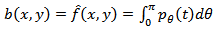 | (3) |
3.1. Back-projection Algorithm (BP)
Backprojection represents the accumulation of the ray-sums of all the rays that pass through any point. Applying backprojection to projection data is called the summation algorithm. In ideal conditions (in particular, without attenuation), the projections acquired at angles between  radians (180°) and
  radians (360°) do not provide new information, because they are only the symmetric of the projections acquired at angles between 0 and
  . This is why the bounds of the integral are limited between 0 and
  radians. The main point of this part is that the backprojection operation is not the inverse of the projection operation. This means that applying backprojection to the function
  does not yield
  but a blurred
  as it will be shown in our simulation results.
3.2. Filtered Back-projection (FBP) Algorithm
It is possible to derive reconstruction algorithms from the so-called Fourier slice theorem [8]. This theorem relates the Fourier transform of a projection to the two-dimensional Fourier transform of the object which is to be reconstructed. Thus given the Fourier transform of a projection at enough angles the projections could be assembled into a complete estimate of the two dimensional transform and then simply inverted to arrive at an estimate of the object. The algorithm that is derived by using the Fourier Slice Theorem is the Filtered Back Projection algorithm. It has been shown to be extremely accurate and amenable to fast implementation. The FBP can be understood as follows: each line of the sinogram is filtered first in order to decrease the blur of the reconstructed image obtained by BP, and the filtered projections are backprojected. This is mathematically expressed as: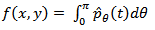 | (4) |
Where  is the filtered version of
  with the ramp filter which gives a weight proportional to its frequency to each of the components. So, the relationship between
  and
and  is expressed as
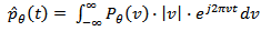 | (5) |
Where  is 1D Fourier Transform of
 , multiplying with
  gives ramp filtering, integrating the expression from
  to
to  gives inverse 1D Fourier Transform. Substituting (5) in (4), yields:
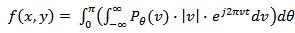 | (6) |
Therefore, the complete Filtered Back Projection algorithm can be viewed in Figure 3.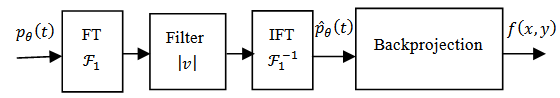 | Figure 3. Filtered Back Projection algorithm |
Notice that analytical reconstruction methods work well when we have a great number of projections uniformly distributed around the object and cannot give satisfactory results when the number of projections is less than thirty two as it will be shown in our simulation results:
4. Iterative Reconstruction Methods
Computed tomography using iterative reconstruction techniques is viewed as a linear inverse problem as follows: find a vector  , that is a solution of
  . So, the principle is to find a solution by successive estimates. In order to implement these algorithms, we first make an initial guess
  at the solution. Then we take successive projections. The projections corresponding to the current estimate are compared with the measured projections. The result of the comparison is used to modify the current estimate, thereby creating a new estimate. The algorithms differ in whether the correction is carried out under the form of an addition or a multiplication.
4.1. Algebraic Reconstruction Methods
The mathematical formulation of the reconstruction problem is posed as a system of linear equations [8], which should be solved when reconstructing an image: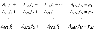 | (7) |
So we write the set of linear equations for each ray as: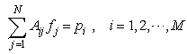 | (8) |
Where  are projection data along the
  ray. In other words, the projection at a given angle is the sum of non-overlapping, equally wide rays covering the figure,
  is the total number of rays (in all the projection).
  are the weights that represent the contribution of every pixel for all the different rays in the projection.
  are the values of all the pixels in the image and
  is the total number of the pixels in the image. In applications requiring a large number of views and where large-sized reconstructions are made, the difficulty with using (8) can be in the calculation, storage, and fast retrieval of the weight coefficients
  , also the dimensions of the matrix
  become so large that direct factorization methods become infeasible, which is usually the case in two and three dimensions. This difficulty can pose problems in applications where reconstruction speed is important. In this case, one can use iterative methods for solving (8), which are described in brief as follows.
4.1.1. Algebraic Reconstruction Technique (ART)
The ART is sequential method, i.e., each equation is treated at a time, since each equation is dependent on the previous. The equation of ART is given by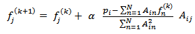 | (9) |
Where  are the current and the new estimates, respectively;
  is the sum weighted pixels along ray
  for the
  iteration;
  is the measured projection for the
  ray , and
  is the relaxation parameter. The second term on the left in equation (9), is the term of correction. The process starts by making an intialguess. Observing equation (9), we see that (a) this correction term is added to the current estimate in order to found the new estimate and (b) the comparison consists in the subtraction of the estimated projections from the measured projections. Also, we can easily see, that equation (9) is used to update the value of the
  pixel on every ray equation. This process can be summarized in Figure 4. Notice that the role of the relaxation parameter
  is to reduce the effects of the noise which is caused by poor approximations of the ray-sums.
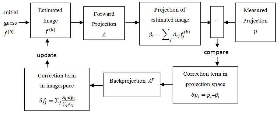 | Figure 4. Algebraic Reconstruction Technique |
4.1.2. Simultaneous Iterative Reconstruction Techniques (SIRT)
As the name refers to, all the methods of this class are simultaneous, which means that information from all the equations are used at the same time. In this approach, we go through all the equations, and then only at the end of each iteration are the pixel values changed, the change for each pixel being the average value of all the computed changes for that pixel. This constitutes one iteration of the algorithm. In the second iteration, we go back to the first equation in (7) and the process is repeated. The SIRT algorithm has however not gained a wide popularity, because it has a big downside. SIRT appears to require a long time for convergence and thus takes a long time for reconstructing an image. For this reason SART or Simultaneous ART was developed.
4.1.3. Simultaneous Algebraic Reconstruction Techniques (SART)
As well known, simultaneous algebraic reconstruction technique (SART) was proposed as a major refinement and an enhanced version of ART since it is a combination of the positive aspect of SIRT and ART [8]. The equation for iterative process using SART can be represented as below: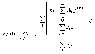 | (10) |
We can easily see, from equation (10), that the correction term, is additive. The main difference between ART and SART is that the correction terms in SART are simultaneously applied for all the rays in one projection, whereas the pixel values are updated ray-by-ray in ART. This explains why SART converges faster than ART.In the following we will discuss Gradient algorithm and Bayesian maximum a posteriori (MAP) approach. Both are optimization methods, that is, they find the best estimate for the solution fitting a given criterion; in the Gradient algorithm, the criterion is the minimization of the difference between  and
and  , whereas in the Bayesian (MAP) approach, which is based on Bayes’ formula as the name refers to, the criterion is the maximization of an associated objective function of the reconstructed image.
4.2. Gradient Algorithm
In iterative methods, one wants to solve  . Where
  is the vector of values in the sinogram,
  is a given matrix, and
  is the unknown vector of pixel values in the image to be reconstructed. One of the iterative reconstruction techniques is the Gradient algorithm. The Gradient algorithm or steepest-descent algorithm iteratively searches for
  using the equation:
 | (11) |
This means that the new estimate  is equal to previous estimate
  plus a second term indicating the new direction (chosen to be opposite to the local gradient, and therefore directed toward the steepest-descent), weighted by a coefficient
  representing the step length. This coefficient can be chosen to optimize the convergence of the process. As we can see from equation (11), the correction factor, which is the second term, is additive. The Gradient algorithm consists essentially of four steps:• Compute
  (Forward projection)• Compute
  (Error or residual)• Distribute
  (Backprojection of error)• Update
  The criterion of this optimization algorithm is the progressive minimization of the difference between the measured projections and estimated ones. That is, the error is defined as:
  In general, reconstruction problem is an ill posed inverse problem. There is immense need for prior information. However, The Gradient method, which is a deterministic regularization process, does not have enough tools to account for stronger prior information needed in some applications. For this reason, probabilistic methods have been developed. One of these probabilistic methods is Bayesian approach which will be described in the following.
4.3. Bayesian Approach
The goal is to find  with respect to two requirements: (a) estimated projections have to be as close as possible to measured projections and (b) the reconstructed images have to be not too noisy. Therefore, the introduction of a prior knowledge as constraint, may considerably favor convergence of iterative algorithms. This process is called regularization. The prior, based on an assumption of what the true image is, is usually chosen to penalize the noisy images. We consider the linear model with additive white Gaussian noise, i.e.,
 | (12) |
Where  and
and  are vectors of random variables. In Bayesian inversion theory, the complete solution for an inverse problem is represented by the posterior distribution, given by Bayes’ formula
 | (13) |
Where  is the likelihood density,
  is the prior density and
  is normalization constant. We select the maximum a posteriori (MAP) estimate which is obtained from
 | (14) |
It means that for the given prior density  and the measurement data
  , we determine the unknown values
  which are in the best agreement with the model (12). Assuming zero mean, isotropique Gaussian noise with variance
  the likelihood function is
 | (15) |
The next question is how to choose the prior density function  . For the sake of clarity, we select the Gaussian white noise prior with the positivity constraint, i.e.,
 | (16) |
Where the step function  equals to one when all the elements in
  are positive; otherwise it is zero. The computation of MAP implies minimizing
 | (17) |
Where the regularization parameter  The higher the noise level, the larger the regularization parameter
  The statistical estimation problem is hence converted into an optimization problem. In other words, at each iteration
  a current estimate of the image is available. Using a system model (which may include attenuation and blur), it is possible to simulate what projections of this current estimate should look like. The measured projections are then compared with simulated projections of the current estimate, and the error between these simulated and measured projections is used to modify the current estimate to produce an updated (and hopefully more accurate) estimate, which becomes iteration
  This process is then repeated many times. In practice, the MAP-estimate is computed by minimum norm least square (MNLS) iterative method implemented in Matlab Optimization Toolbox. But, Bayesian approach is not only limited to MAP estimator. Many other estimators have been proposed such as the Posterior mean and Marginal MAP estimator. So, the main steps in Bayesian approach are (a) prior density modeling (which can be Gaussian, Generalized Gaussian, Gamma mixture, etc. ... .) and (b) the choice of the estimator and computational aspects. The most important advantage of Bayesian approach is that it is a coherent approach to combine information content to the data and priors.
5. Reconstruction Quality, in the Context of Computational Performance
The BP, FBP, Gradient and Bayesian algorithms are implemented and tested for two test images. These algorithms have been implemented on a PC using Matlab programming language. In order to objectively evaluate the reconstructed results, we have computed four image quality measurement parameters proposed in [3] in addition to two relative norm errors and the visual quality of the reconstructed image. The quality measurements are listed below:The relative norm error of the resulting images [8] is used and defined as: | (18) |
Where  is the gray level value of the test image and
  is the gray level value of the reconstructed image. The relative norm error of the simulated projections and defined as
 | (19) |
Where  is the measured projection and
  is the simulated projection.Mean square error
  it’s measure between the test image and the reconstructed image and defined as:
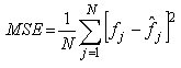 | (20) |
Where  is the value of the pixel in the test image
  and the value of the pixel in the reconstructed image,
  is the total number of pixels.Normalized cross-correlation
  is defined as:
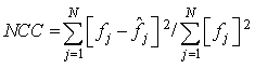 | (21) |
Smaller errors  and
and  , means that the resulting reconstructed image is closer to the test image.Structural content
  it’s the measure of image similarity based on small regions of the images containing significant low level structural information and is defined as:
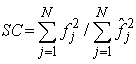 | (22) |
Peak Signal to Noise Ratio  is defined as:
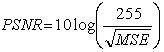 | (23) |
Another criterion for the iterative reconstruction techniques is the number of iterations. Smaller iteration is preferable. Projections (parallel beam type) for the image reconstruction are calculated analytically by defining the first test image: Shepp-Logan phantom head model (Simulated) image as it is shown in Figure 2. Figure 5 shows the second test image which is the standard medical image of abdomen. Projections are calculated mathematically. The two original test images are grayscale images of size  and
and  respectively, with coverage angle ranging from 0° to 180°with rotational increment of 10° to 2°.
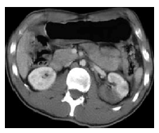 | Figure 5. Input test image: Standard medical image of abdomen |
6. Results and Discussion
Comparison of reconstruction techniques such as BP, FBP (analytical), Gradient and Bayesian algorithm (iterative) with respect to performance parameters and visual quality of reconstructed images is presented in this section. The reconstruction performances are calculated versus number of projections and number of iterations. Figure 6 shows the reconstruction of 2D Shepp-Logan phantom head model (Figure 2) by BP with different projections. The simulated Peak Signal to Noise Ratio PSNR results as well as Figure 7 show that minimum 64 projections, with coverage angle ranging from 0°to 180° with an incremental value of 3° is necessary to reconstruct the image with acceptable quality. This technique generates star or spoke artifact. Figures 6 and 7 clearly reveal that the quality of reconstructed image slightly increases as number of projections increases. The reconstructed images appear to be very blurry. The quality measurements versus projections of Shepp-Logan image using BP are drawn in Figure 8. The later reveals very close similarity among computational performance with the visual quality of reconstructed image shown in Figure 6.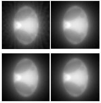 | Figure 6. Reconstructed image of Shepp-Logan phantom by BP. Using (a) 16, (b) 32, (c) 64 and (d) 180 number of projections (from left to right, up to bottom) |
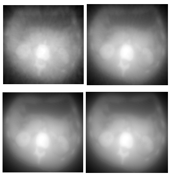 | Figure 7. Reconstructed image of standard medical image by BP using 16, 32, 64 and 180 number of projections (from left to right, up to bottom) |
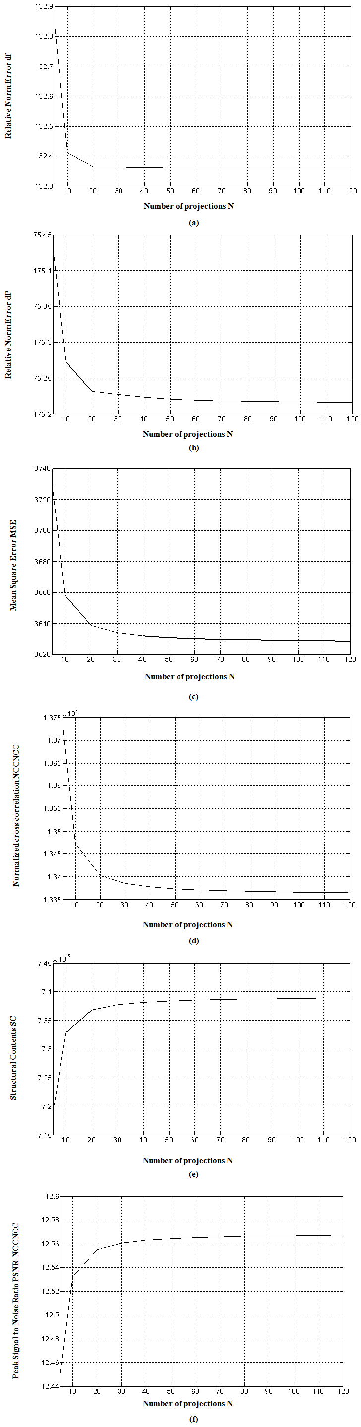 | Figure 8. Quality measurements v/s number of projections for BP. (a)  (b) (b)  (c) (c)  (d) (d)  (e) (e)  (f) (f)  .Test image: Shepp-Logan .Test image: Shepp-Logan |
Figure 9 shows the reconstruction of phantom head model and the standard medical of abdomen by FBP with coverage angle ranging from 0°to 180°with an incremental value 10° of to 2°. Figure 9 clearly reveals that the quality of reconstructed images of both Shepp-Logan phantomand the standard medical image of abdomen increases as number of projections increases. The graphical representation of quality measurements versus projections of Shepp-Logan test Image for FBP is shown in Figure 10.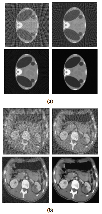 | Figure 9. Reconstructed image of (a) Shepp-Logan phantom (b) standard medical image, by FBP (with Shepp-Logan filter).Using 16, 32, 64 and 180 number of projections (from left to right) |
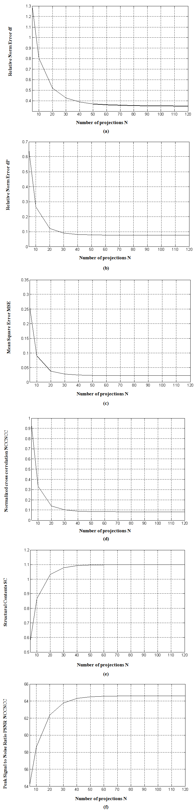 | Figure 10. Quality measurements v/s number of projections for FBP with Hanning filter. (a)  (b) (b)  (c) (c)  (d) (d)  (e) (e)  (f) (f)  .Test image: Shepp-Logan .Test image: Shepp-Logan |
We can easily observe that the performance parameters remain almost constant after 32 projections. This algorithm requires a minimum of about 32 projections with rotational increment of 5° to display acceptable reconstructed image. It is the most common method of removing the star artifact which is normally generated in BP by using various filters. FBP algorithm is fast and efficient with large number of projections. Also after about 32 projections, trend of errors appear to decrease consistently, unlike  which significantly increases after 32 projections. Table 1 shows the quality measurements by varying the filter used in FBP and keeping common number of projections.
 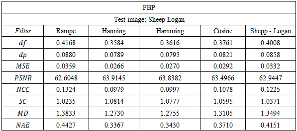 | Table 1. Quality measurements by varying the filter keeping fixed number of projections (32) |
Table 1 demonstrates that the quality measurements, from FBP using Hanning filter are slightly better than those of other filters. This means that the choice of the filter has not a significant effect to enhance the image quality. From Figure 11, it can be clearly seen that visual quality of the reconstructed images for various filters is almost similar.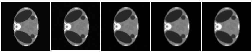 | Figure 11. Reconstructed images by FBP. Using (a) Ramp, (b) Shepp-Logan, (c) Cosine, (d) Hamming and (e) Hanning filters, number of projections 180 |
The resultant reconstructed images obtained from Gradient algorithm by varying the number of iterations, are shown in Figure 12. The later demonstrates that Gradient algorithm is providing better reconstruction than that of FBP and BP. The quality measurements versus projections of Shepp-Logan image using Gradient algorithm for 200 iterations are shown in Figure13. We can easily observe that performance parameters are considerably enhanced comparatively with those of FBP especially for low number of projections, since error values obtained from Gradient algorithm are significantly reduced with a significant increase of  . We should note here that the number of iterations is much required in order to enhance the image quality.
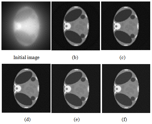 | Figure 12. Reconstructed images by Gradient algorithm. Using (b) 20, (c) 60, (d) 100 (e) 200 and (f) 500 iterations |
 | Figure 13. Quality measurements v/s number of projections for Gradient algorithm. Using 200 iterations (a)  (b) (b)  (c) (c)  (d) (d)  (e) (e)  (f) (f)  . Test image: Shepp-Logan . Test image: Shepp-Logan |
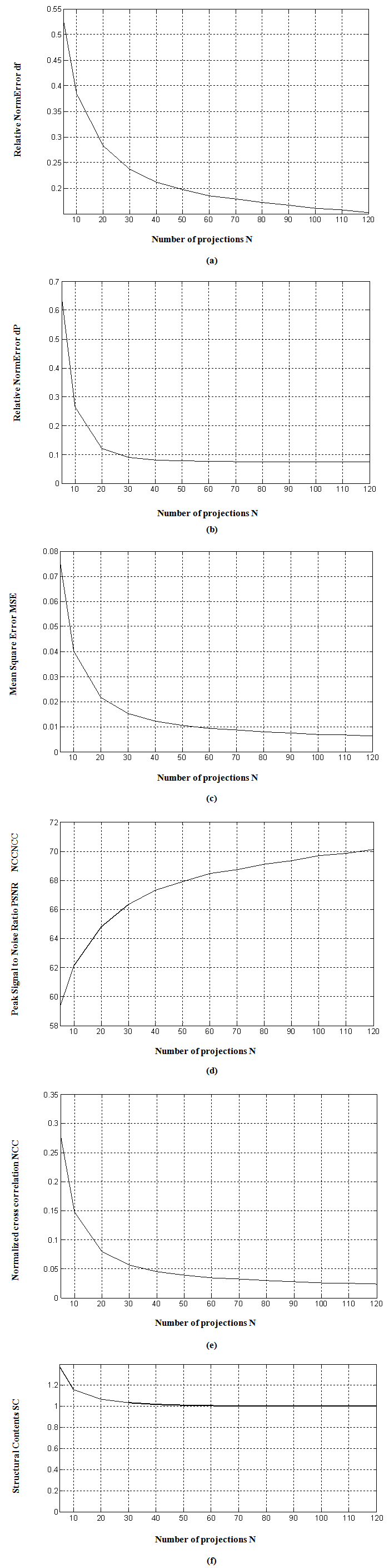
Figure 14 shows the resultant reconstructed images obtained from Bayesian algorithm by varying the number of iterations. Figure 15 shows the quality measurements versus projections, obtained from Bayesian algorithm keeping common number of iterations  The experiments reveal the fact that Bayesian algorithm effectively eliminated Star artifacts created by BP. The quality measurements are significantly enhanced comparatively with those of Gradient and FBP techniques.
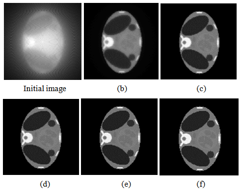 | Figure 14. Reconstructed images by Bayesian algorithm using (b) 20, (c) 60, (d) 100, (e) 200 and (f) 500 iterations |
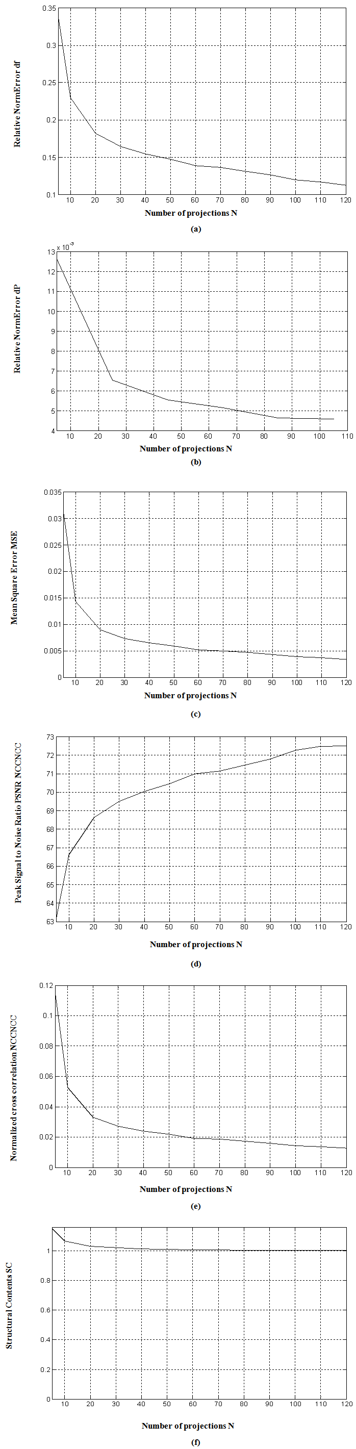 | Figure 15. Quality measurements v/s number of projections for Bayesian algorithm. Using 200 iterations (a)  (b) (b)  (c) (c)  (d) (d)  (e) (e)  (f) (f)  . Test image: Shepp-Logan . Test image: Shepp-Logan |
To more illustrate the benefits of the Bayesian approach, we provide Figure 16, Tables 2 and 3 which compare the quality measurement parameters obtained via reconstruction techniques discussed in this work. Table 4 shows the difference between Gradient and Bayesian algorithms of Shepp-Logan phantom in term of performance parameters using 100 and 200 iterations. Bayesian algorithm performs better even at limited number of projections as shown in Figure 16, and has better quality of reconstruction.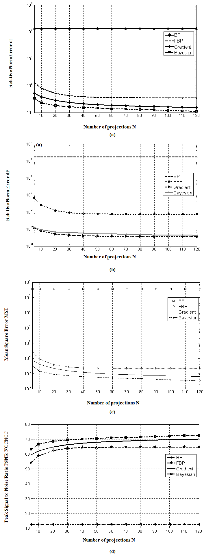 | Figure 16. Comparison of reconstruction techniques. In term of (a)  (b) (b)  (c) (c)  (d) (d)  with different projections and common number of iterations for Gradient and Bayesian algorithms (200). Test image: Shepp-Logan with different projections and common number of iterations for Gradient and Bayesian algorithms (200). Test image: Shepp-Logan |
The experiments revealed major observations; as the number of projections within a given angular range was increased, the quality of reconstructed image appeared better for both analytical and iterative algorithms. The errors  and
and  obtained from the Bayesian algorithm are less than those of BP, FBP and Gradient algorithms. A high value of
  is obtained via Bayesian algorithm. Also, the star artifact appearing in image reconstructed from the Filtered Back Projection is disappeared with the method of Gradient and Bayesian algorithms. However, Gradient and Bayesian algorithms take more time to complete the process than does FBP. But for smaller number of projections, time is almost equal for both Gradient and Bayesian algorithms. Results obtained using Mat lab (The Math Works, Inc., Natick, MA), version 7.10 (R2010a), under the Window XP operating system (Microsoft Corp., Redmond, WA), on Intel Pentium Core2 Duo, CPU 3 GHz, 1.93 GB RAM. It was found, for both analytical and iterative methods studied in this work that the quality measurements except
  and
and  , decreased with increasing number of projections. We can clearly observe, from Tables 2, 3 and 4, that lower values for
  , which it means lesser error, correspond to high values of
  . Logically, a higher value of
  is good because it means that the ratio of Signal to Noise is higher. Here, the 'signal' is the test image, and the 'noise' is the error in reconstruction. The number of iterations in the case of Gradient and Bayesian algorithms is much required in order to enhance the image quality.
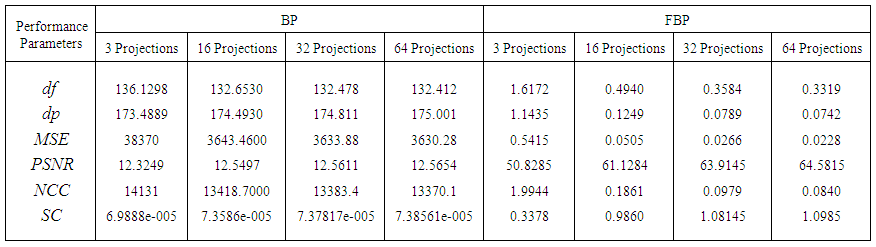 | Table 2. Performance parameters by varying number of projections for reconstruction techniques. Test image: Shepp-Logan |
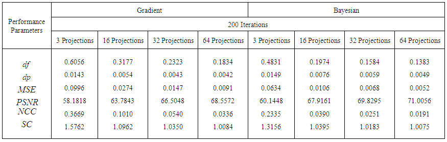 | Table 3. Performance parameters by varying number of projections for reconstruction techniques. Test image: Shepp-Logan |
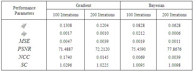 | Table 4. Performance parameters by varying number of iterations for Gradient and Bayesian approach. Test image: Shepp-Logan |
7. Conclusions
This paper presents the comparisons of the image reconstruction algorithms using BP, FBP analytical methods, Gradient and Bayesian iterative algorithms. In this work, objective measurement by six performance parameters, led to an ability to subjectively judge the reconstructed image quality. By Gradient and Bayesian algorithms, the problems in star artifacts, the quality measurements and the reconstructed image quality can be significantly improved. The results show that Bayesian method provides the best image quality, small values of the errors  and
and  and high values of
  especially for large number of iterations. From the simulated results, we shall conclude that the Bayesian algorithm is reliable and practical to enhance the quality of reconstructed images and more suitable method for CT applications.
ACKNOWLEDGEMENTS
We thank M.A Djafari for inspiring discussions and explanation of Bayesian theory during the short stay of Z. Messali in Supelec, France 2011 and for giving her useful feedback on this work.
References
| [1] | Q. Zhong, W. Junhao, Y. Pan, “Algebraic Reconstruction Technique in Image Reconstruction with Narrow Fan Beam,” IEEE Trans. Medical Imaging., 52(5), pp.1227-1235, 2005. |
| [2] | L. Bao-dong, L. Zeng, J. Dong-jiang, “Algebraic Reconstruction Technique Class for Linear Scan CT of Long Object,” In. Proc. the 17th World Conference on Nondestructive Testing., Shanghai, China,Oct. 2008. |
| [3] | Desai, S. D., Kulkami, L., 2010, A Quantitative Comparative Study of Analytical and Iterative Reconstruction Techniques., International Journal of Processing (IJIP), 4(4), pp. 307-319. |
| [4] | Anishinraj, M.M., Venkataraman, B., Vaithiyanathan, V., 2012, A Comparative Study and Experimentation of Simultaneous Algebraic Reconstruction Technique (SART) and Ordered Subsets Expectation Maximization (OSEM)., Eur. J. Sci. Res., 4(68) , pp. 584-590. |
| [5] | V.H. Tessa, W. Sarah, G. Maggie, B.K. Joost, S. Jan, “The implementation of Iterative Reconstruction Algorithms in MATLAB,” Master Thesis, Department of Industrial Sciences and Technology, University College of Antwerp, Belgium, July. 2007. |
| [6] | Philippe. P.B., 2002, Analytic and Iterative Reconstruction Algorithms in SPECT., J. Nucl Med. 43(10), 1343-1358. |
| [7] | Andersen, A.H., Kak, A.C., 1984, Simultaneous Algebraic Reconstruction Technique (SART) A Superior Implementation of the ART algorithm, Ultrasonics Imaging, 6(1),81–94. |
| [8] | A.C. Kak, M. Slaney, “Principles of computerized tomographic imaging,” IEEE Press., 1988. |
| [9] | D. Raparia, J. Alessi, A. Kponu, “The Algebraic Reconstruction Technique (ART),” Ph.D. dissertation, AGS Department, Brookhaven National Lab, Upton, NY 11973, USA, 1997. |
| [10] | H. Carfanton, A.M. Djafari, “A Bayesian Approach For Nonlinear Inverse Scattering Tomographic Imaging,” Proceedings of IEEE ICASSP., vol. 4, pp. 2311-2314, USA, 1995. |
| [11] | T. Hebert, R. A. Leahy, “Generalized EM Algorithm For 3-D Bayesian Reconstruction From Poisson Data Using Gibbs Priors,” IEEE Trans. Med Imaging., vol. 8, pp.194-202, 1989. |
| [12] | L. T. Hsiao, A. Rangarajan, G. Gindi, “Joint-Map Reconstruction/ Segmentation for Transmission Tomography Using Mixture-Models as Priors,” Proc IEEE Nuclear Science Symposium and Medical Imaging Conference., vol.3,pp. 1689-1693,Toronto, Canada ,Nov. 1998. |
| [13] | C. Soussen, A. M. Djafari, “Closed Surface Reconstruction in X-Ray Tomography,” Proc IEEE Int Conf Image Processing., vol.1, pp.718–721, Thessaloniki, Greece, Oct. 2001. |
 Abstract
 Reference
 Full-Text PDF
 Full-text HTML