Peeyush Misra, R. Karan Singh
Department of Statistics, Lucknow University, Lucknow, India
Correspondence to: Peeyush Misra, Department of Statistics, Lucknow University, Lucknow, India.
| Email: |  |
Copyright © 2015 Scientific & Academic Publishing. All Rights Reserved.
Abstract
For estimating finite population variance using information on single auxiliary variable in the form of mean and variance both, the Ratio-Product-Difference (RPD) type estimators are proposed. The generalized cases of these estimators leading to the classes of estimators are also proposed. The bias and mean square error (MSE) of the proposed estimators are found. Theoretical comparisons with the traditional estimator are supported by a numerical example. By this comparison it is shown that the proposed estimators are more efficient than the traditional one.
Keywords:
Auxiliary Variable, Taylor’s Series Expansion, Bias, Mean Square Error (MSE) and Efficiency
Cite this paper: Peeyush Misra, R. Karan Singh, Estimators for Finite Population Variance Using Mean and Variance of Auxiliary Variable, International Journal of Probability and Statistics , Vol. 4 No. 1, 2015, pp. 1-11. doi: 10.5923/j.ijps.20150401.01.
1. Introduction
In sampling theory, auxiliary information is used widely at both the stages of selection and estimation. At the estimation stage, auxiliary information is used by formulating various types of estimators of different population parameters with a view of getting increased efficiency and are available in plenty in the literature.Let U = (1, 2, . . . , N) be a finite population of N units with Y being the study variable taking the value  for the unit i of U and X being the auxiliary variable taking the value
  for the unit i of the population, i = 1, 2, . . . , N.Let
  be the population of mean of Y and
  be the population mean of X. Also, let
 ,
, and
and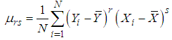 For a simple random sample of size n drawn from U with the sample observations
  ,
,  , . . . ,
  on
on  and
and  ,
, , . . . ,
  on
on  , let
, let  and
and  be the sample means of y-values and x-values respectively.
2. The Suggested Estimators
We know that the finite population variance  of the study variable is
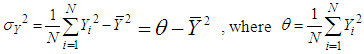 | (2.1) |
From (2.1) it is natural to get an estimator of  if we replace
  and
and  by their some estimators. In particular if
  is estimated by
  and
and  is estimated by
 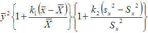 , we get the estimator of
  as follows
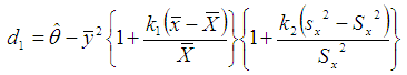 | (2.2) |
and its generalized estimator as  | (2.3) |
where  and
and  and f (u , v) satisfying the validity conditions of Taylor’s series expansion is a bounded function of (u , v) such that f(1, 1) = 1.Also if
  is estimated by
  and
and  is estimated by
  , we get another estimator of
  as follows
 | (2.4) |
and its generalized estimator as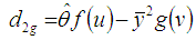 | (2.5) |
where  and
and  , f(u) and g (v) both are bounded functions in u and v respectively such that
  = 1 at the point u = 1 and
  = 1 at the point v = 1 and both are satisfying the regularity conditions for the validity of Taylor’s series expansion having first two derivatives with respect to u and v respectively to be bounded.
3. Bias and Mean Squared Error of Suggested Estimators
(a) Bias and Mean Square Error of Suggested Estimator  Let
Let  ,
,  ,
, 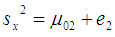 and
and  ,For simplicity, it is assumed that the population size N is large enough as compared to the sample size n so that finite population correction terms may be ignored. Now
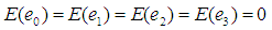 | (3.1) |
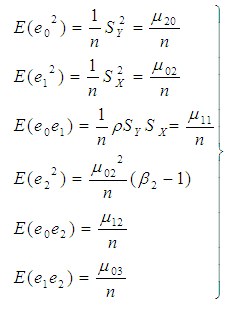 | (3.2) |
and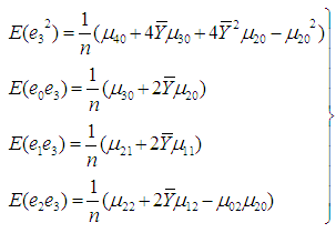 | (3.3) |
Let us consider the proposed estimator  defined in (2.2)
 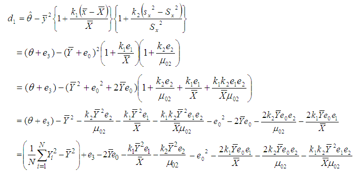 or
or | (3.4) |
Taking expectation on both sides of (3.4), the bias in 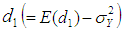 to the order
  is given byBias
 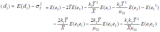 Using values of the expectations given from (3.1) to (3.3), we have
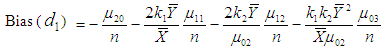 | (3.5) |
Now squaring (3.4) on both sides and then taking expectation, the mean square error of 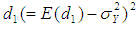 to the first degree of approximation is given by
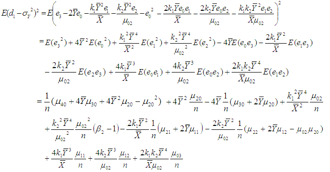 or
or 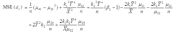 | (3.6) |
For minimizing (3.6) in two unknowns  and
and  , the two normal equations after differentiating (3.6) partially with respect to
  and
and  are
are 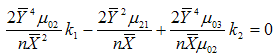 | (3.7) |
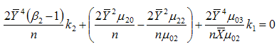 | (3.8) |
Solving (3.7) and (3.8) for  and
and  , we get the minimizing optimum values to be
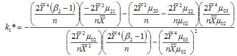 | (3.9) |
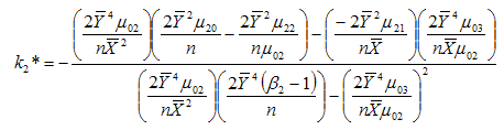 | (3.10) |
which when substituted in (3.6) gives the minimum value of mean square error of the estimator  as
as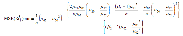 | (3.11) |
(b) Bias and Mean Square Error of Suggested Estimator  For f1 and f2 being the first order partial derivatives of
  with respect to u and v respectively at the point (1,1), that is
 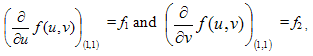 expanding
  in (2.3) in third order Taylor’s series about point (1, 1), we have
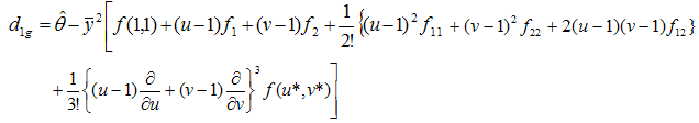 where f1 and f2 are already defined; f11, f22 and f12 are the second order partial derivatives given by
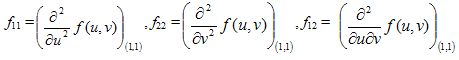 and u* = 1 + h ( u- 1) , v *= 1 + h ( v-1) , 0 < h < 1.or
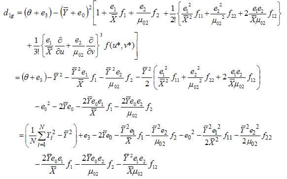
 | (3.12) |
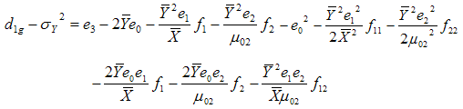
Taking expectation on both sides of (3.12) and using values of the expectations given from (3.1) to (3.3), the bias in 
 to the order
  is given by
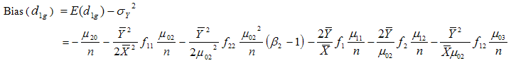
 | (3.13) |
Now squaring (3.12) on both sides and then taking expectation, the mean square error of  to the first degree of approximation is given by
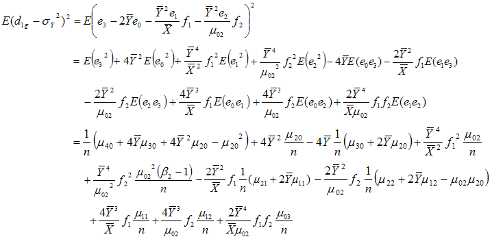
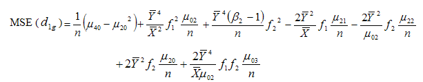 | (3.14) |
For minimizing (3.14) in two unknowns f1 and f2 , the two normal equations after differentiating (3.14) partially with respect to f1 and f2 are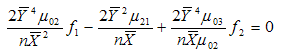 | (3.15) |
 | (3.16) |
Solving (3.15) and (3.16) for f1 and f2, we get the minimizing optimum values to be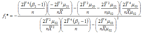 | (3.17) |
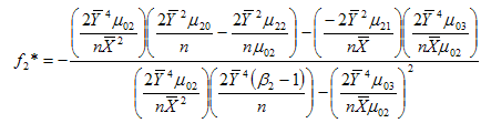 | (3.18) |
which when substituted in (3.14) gives the minimum value of mean square error of the estimator  as
as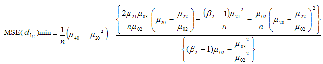 | (3.19) |
(c) Bias and Mean Square Error of Suggested Estimator  Let us consider the proposed estimator
  defined in (2.4)
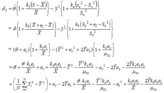 or
or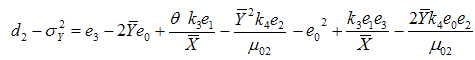 | (3.20) |
Taking expectation on both sides of (3.20), the bias in 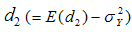 up to terms of order
  is given by
 Using values of the expectations given from (3.1) to (3.3), we have
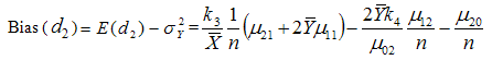 | (3.21) |
Now squaring (3.20) on both sides and then taking expectation, the mean square error to the first degree of approximation is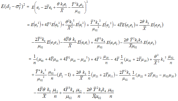 or
or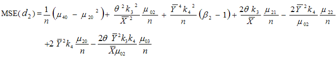 | (3.22) |
For minimizing (3.22) in two unknowns  and
and  , the two normal equations after differentiating (3.22) partially with respect to
  and
and  are
are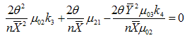 | (3.23) |
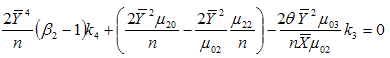 | (3.24) |
Solving (3.23) and (3.24) for  and
and  , we get the minimizing optimum values to be
 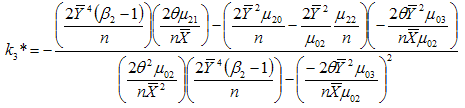 | (3.25) |
and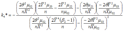 | (3.26) |
which when substituted in (3.22) gives the minimum value of mean square error of the estimator to be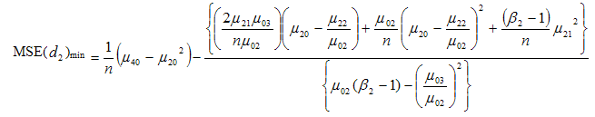 | (3.27) |
(d) Bias and Mean Square Error of Suggested Estimator  For
For  ,
,  and
and  to be first, second and third order derivatives of
  at the point u = 1, u* = 1 + h1 (u-1), 0 < h1 < 1 , also
  ,
,  and
and  to be first, second and third order derivatives of
  at the point v = 1 and v* = 1 + h2 (v-1), 0 < h2 < 1, expanding
  and
and  in
in  in third order Taylor’s series, we have
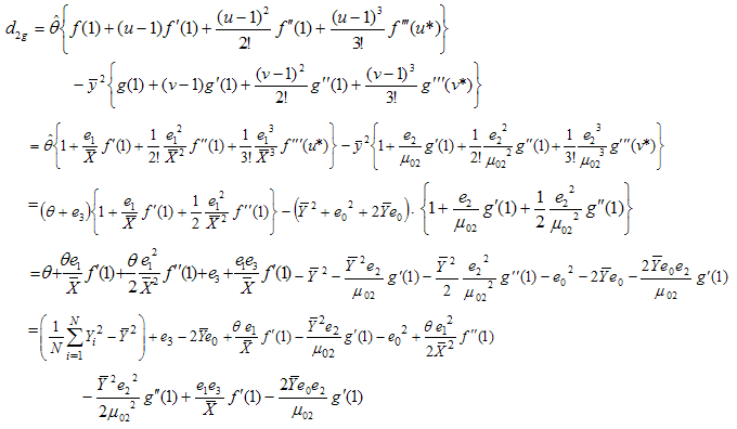 or
or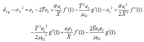 | (3.28) |
Taking expectation on both sides of (3.28) and using values of the expectations given from (3.1) to (3.3), the bias in 
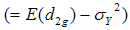 to the order
  is given by
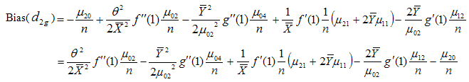 | (3.29) |
Now squaring (3.28) on both sides and then taking expectation, the mean square error of  to the first degree of approximation is given by
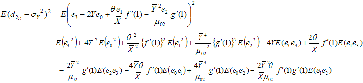 Using values of the expectations given from (3.1) to (3.3), we have
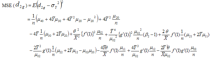 or
or 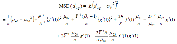 | (3.30) |
For minimizing (3.30) in two unknowns  and
and  , the two normal equations after differentiating (3.30) partially with respect to
  and
and  are
are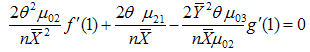 | (3.31) |
and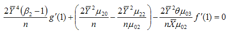 | (3.32) |
Solving (3.31) and (3.32) for  and
and  , we get the minimizing optimum values to be
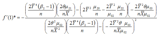 | (3.33) |
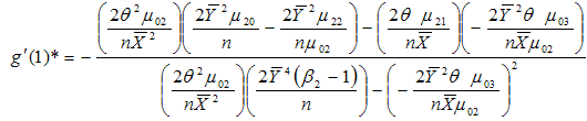 | (3.34) |
which when substituted in (3.30) gives the minimum value of mean square error as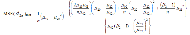 | (3.35) |
4. Efficiency Comparison with the Traditional Estimator
As we know that the mean square error of usual conventional unbiased estimator  of population variance
  is
is  and
and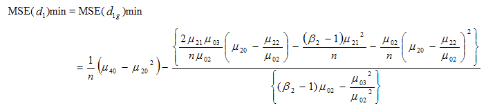 | (4.1) |
and 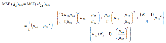 | (4.2) |
Comparative studies regarding their efficiency over the usual conventional unbiased estimator are carried out with the help of a numerical illustration.Considering the data given in Cochran (1977) dealing with Paralytic Polio Cases ‘Placebo’ (Y) group, Paralytic Polio Cases in not inoculated group (X), computations of required values of  have been done and comparisons are made for a simple random sample of size n. For the data considered, we have
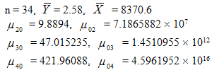
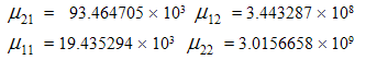 Using above values, we haveMean Square Error of usual conventional unbiased estimator = 9.534136695 and
 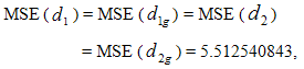 Hence the percent relative efficiency (PRE) of the proposed estimators
  ,
,  ,
,  , and
, and  over the usual conventional estimator are given by
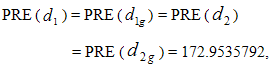 showing that the proposed estimators
  ,
,  ,
,  , and
, and  are more efficient with highly significant percent relative efficiency over the usual conventional unbiased estimator of the population variance.
5. Conclusions
We have derived new sampling estimators of population variance using auxiliary information in the form of mean and variance both, the bias and mean square error equations are obtained. Using these equations, MSE of proposed estimators are compared with the traditional estimator in theory and shown that the proposed estimators have smaller MSE than the traditional one.
ACKNOWLEDGEMENTS
The authors are thankful to the referees and the Editor- in- chief for providing valuable suggestions regarding improvement of the paper.
References
| [1] | Cochran, W. C. (1977) – ‘Sampling Techniques’, 3rd Edition, John Wiley and Sons, New York. |
| [2] | Das, A. K. and Tripathi, T. P. (1978) – Use of auxiliary information in estimating the finite population variance. Sankhya, Vol. 40, Series C, 139-148. |
| [3] | Singh, R. K., Zaidi, S. M. H. and Rizvi, S. A. H (1995) – Estimation of finite population variance using auxiliary information, Journ. of Statistical Studies, Vol. 15, 17-28. |
| [4] | Singh, R. K., Zaidi, S. M. H. and Rizvi, S. A. H.(1996) – Some estimators of finite population variance using information on two auxiliary variables., Microelectron, Reliab., Vol. 36, No. 5, 667-670. |
| [5] | Srivastava, S. K. and Jha, J. J. H. S. (1980) – A class of estimators using auxiliary information for estimating finite population variance, Sankhya, Vol. 40, Series C, 87-96. |
 Abstract
 Reference
 Full-Text PDF
 Full-text HTML