1. Introduction

Target tracking is an important component of many modern applications, including: robots localization, visual tracking, radar tracking, and satellite navigation. In addition, it involves tracking of an object (typical examples include ships, planes and other moving vehicles). The key to a successful target tracking depends on an effective extraction of the useful information about the target state from available observations.

From a Bayesian perspective, the tracking problem can be solved by recursively calculating some degree of belief in the target state, taking different values, given available observations. Thus, it is generally required to construct the conditional probability density function (PDF) of the target state. Since the target state uncertainty and the measurement-originated uncertainty are the two major unavoidable obstacles for target tracking, a good model of the target motion will effectively facilitate the design of the required tracking algorithm. Assume the target motion and its measurements can be reasonably represented by some known mathematical models; the commonly used models are the state space model described in the following form:

(1)

(2)

where and are either linear or nonlinear functions, and represent i.i.d process and measurement noise sequence, respectively. and denote the target state vector and the measurement at sample time , respectively. Models represented by (1) - (2) are referred to as state space model. This includes such models as the bearings-only tracking.

The aim of Bayesian tracking is to estimate recursively conditional PDF using prediction and an updating procedure as follows:

Using (1) to obtain the predictive PDF of for a known PDF at time :

prediction:

(3)

At time , the predictive PDF (3) is updated by the information contained in the measurement through Bayesian Formula:

updating:

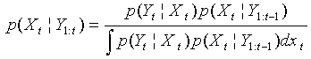(4)

where the normalizing constant is calculated and which depends on the Likelihood function of .

The recurrence relationships in (3) and (4) form the basis of Bayesian tracking. In general, such recursive propagation of the density is generally difficult to analytically determine their compact mathematical expressions since they require the evaluation of complex high-dimensional integrals.

When the system is linear with a Gaussian noise, the Kalman filter constitutes an optimal Bayesian solution Anderson and Moore (1979). However, for most non-linear non-Gaussian models, it is not possible to compute these distributions in closed-form and we need to employ numerical methods.

The problem of target tracking using bearings-only measurements is a difficult task. The filtering algorithms involve a nonlinear measurement process, which, when linearized, can lead to time-varying parameters, biases as explained by Aidala (1979). The common estimation algorithms used for bearings-only target tracking are: Least Squares (batch and recursive forms), Maximum Likelihood Estimator, Extended Kalman Filter (EKF), and Particle Filters or Bayesian Methods.

Most researchers in the field of bearings-only tracking have concentrated on tracking a nonmanoeuvring target. Due to inherent nonlinearity and observability issues, it is difficult to construct a finite-dimensional optimal filter even for this relatively simple problem. As for the bearings-only tracking of a manoeuvring target, the problem is much more difficult.

Early research focuses mainly on analytical derivations for the observability criteria of the estimation process, and comparisons of the convergence properties and performance of the different types of method used for target tracking. Since bearings-only target estimation involves a non-linear measurement process, several filtering and observability complications arise. Lindgren and Gong (1978) analyze the observability associated with a least-squares estimation approach and show that, for a constant velocity target and a constant velocity vehicle moving in a 2-D plane, the target estimation is unobservable until the vehicle executes a maneuver (change in heading). Kalman Filtering techniques are used by Aidala (1979) and by Nardone, et al., (1984). Since the bearings-only estimation problem involves nonlinear measurements, an EKF approach needs to be used instead of the normal Kalman Filter. The EKF however is sensitive to initialization techniques and measurement errors which can cause early covariance collapse and other filter instabilities Aidala (1979). The moving vehicle trajectory affects the observability and convergence of the target estimation, suggesting that a good trajectory design can reduce filter instability and estimation errors.

A pseudolinear filter formulation is proposed by Aidala and Nardone (1982), which attempts to linearize the dynamics and measurement models. However by linearizing the dynamics the noise becomes non-Gaussian which, when propagated through the filter, causes estimation bias. For the bearings-only tracking problem, the bias is introduced only in the position estimate, and is highly dependent on the geometry of the vehicle maneuvers, once again suggesting that the estimation performance can be improved by proper design of the vehicle trajectory. Comparisons of the properties and performance between several different filtering algorithms are explored by Nardone, et al., (1984). Aidala and Hammel (1983) proposed the modified polar coordinates filter. The filter uses an EKF algorithm with a state vector choice, based on polar coordinates, that attempts to separate the observable and unobservable components of the estimated state by using a different coordinate system. The resulting filter is stable and asymptotically unbiased. The modified polar coordinate filter shows the dependence of the target estimation on the vehicle maneuvers, once again suggesting that the estimation can be improved by designing a good trajectory. De Vlieger (1992) used a piecewise linear model of the target motion and a Maximum Likelihood Estimator approach for target tracking. He uses numerical methods to condition the measurement model to increase the observability of the estimation. Goshen-Meskin and Bar-Itzhack, (1992) derive the observability requirements for piecewise constant linear systems. Tao et al., (1996) shows that for a MLE approach it is important to consider the correlation of the noise, and that ignoring it degrades the performance of the estimation.

Several modifications to the classical estimation algorithms have been explored. Some attempt to smooth the trajectory, within the constraints of a known target behavior model. Others consist of designing multiple filters for different known target scenario and using statistical properties of the innovation to switch between the algorithms. Another approach has been to support multiple Kalman filters simultaneously and develop an estimate by combining all the filters. Later research by Bar-Shalom et al. (2002) has focused on using interacting multiple models (IMM). These algorithms employ a constant velocity (CV) model along with manoeuvre models to capture the dynamic behaviour of a manoeuvring target scenario. Le Cadre and Tremois, (1998) modelled the manoeuvring target using the CV model with Gaussian noise and developed a tracking filter in the hidden Markov model framework.

Particle filtering or Sequential Monte Carlo techniques have also been explored by Liu et al., (2002), Bar-Shalom et al., (2001), Ristic et al., (2004). Particle filters have the advantage of being able to deal with nonlinear systems and non-Gaussian noise models making them particularly well suited to bearings-only tracking. They can also accommodate unknown and stochastic target models making them more versatile than classical filters. However, they require increased computational resources and, for fast convergence, need a fairly accurate description of the measurement likelihood function and a good initial distribution on the estimated target location.

In this paper, the particle filter is developed based on the Student’s-t distribution for nonlinear bearing-only tracking problem and compare with the Mixture of Normal (MoN) based particle filter of Kim and Stoffer (2008). The outline of the remainder of this article is organized as follows: section 2 is a general presentation of the BOT problem. Section 3 gives a succinct analysis of the basic theory of the EM procedure and the SMC methods. The details of the proposed EM–SMC (particle filter) algorithm follow. The implementation of the E-step using a particle filter, and the M-step by fitting a Student’s-t model to the estimated data, are provided as well. Simulation results and application to the real data that confirms the proposed method based on Student’s-t are presented in section 4, while section 5 concludes the work.

2. Bearings-Only Tracking

Bearings-only tracking involves estimating the target states based on angle measurements at a sensor node. The target is assumed to move in the x-y plane and to follow a constant-velocity motion model Bar-Shalom and Fortmann (1988) with a state update period of 1s. The state vector contains the positions and velocities of the object in the directions respectively: , where denotes the sampling period. One possible discretization of this model, is given by Gordon et al., (1993)

(5)

The equation of the observed bearing, , is

(6)

where ,

,

Parameter represents the system noise and is Gaussian distributed with covariance where is a identity matrix. This vector can be thought of as representing the acceleration in the and directions. represents the observed bearing of the object measured by the sensor at time represents a Gaussian measurement noise with mean zero and variance . Before measurements are taken, the particle filter recursion is started with initial state vector in the form of a 4 dimensional Gaussian variable with known mean and covariance matrix. As can be seen, this model is 4 dimensional and nonlinear due to a transcendental function in the observation equation. The particle filters handle these situations efficiently. It has been shown through intense simulations in Gordon et al., (1993), that particle filters are much more efficient for this problem than the traditional EKF. The BOT problem is illustrated in figure 1.

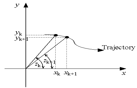Figure 1. The Bearings-Only Tracking (BOT) problem

3. Nonlinear State Estimation Using Expectation-Maximization (EM)

State estimation in a nonlinear state-space dynamical system whose evolution process is described as in equation (1) consists of estimating the state data vector using a sequence of noisy measurements given by the model in equation (2). The main idea in EM-based algorithms is to solve the state estimation problem in the presence of model uncertainty in two iterative steps Baum et al, (1970), Dempster et al. (1977). 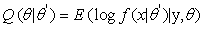Starting from some initial parameters the algorithm iteratively applies:

E-step: Compute the expected likelihood,

M-step: Choose the parameter values that maximizes the function, .

In the E-step, it is assumed that the model is known perfectly and therefore standard estimation methods are used to estimate the states. The primary purpose of the E-step is to estimate the hidden states. This is accomplished by determining the best distribution which makes the expectation of log-likelihood maximum. The M-step involves estimating the model parameters using the states estimated in the previous E-step and their corresponding measurements. Different implementations of the E and the M steps have resulted in different algorithms suitable for different applications.

In the E-step of the proposed algorithm, an approximation of the desired distribution of the states given the measurements is formulated. This distribution is then used to estimate the states. In nonlinear systems this conditional density is generally non-Gaussian and can be quite complex. We use a SMC (particle filter) Doucet et. al. (2001) algorithm to estimate and recursively update this distribution in time. This greatly assists the algorithm in converging to the global optimum. In the maximization (M) step, the unknown measurement process is approximated by fitting the observations to a Student’s-t model using the current estimate of the states.

3.1. Sequential Monte Carlo Methods

After the introduction of SMC in the 1960’s, it has become an emerging methodology for the nonlinear or non-Gaussian state-space models. SMC methods or particle filters are a class of recursive simulation methods for solving filtering problems Doucet et. al., (2001), Gordon et. al., (1993).

The chief initiative is to represent the interested density function at time by a set of random samples with associated weights, and compute estimates based on these samples and associated weights. As the number of samples becomes very large, this Monte Carlo characterization develops into an equivalent representation to the functional description of the posterior probability density function (Arulampalam, et. al., 2002).

If we let be samples and associated weights approximating the density function is a set of particles with associated weights with , then the density function are approximated by

signifies the Dirac delta role. The particle approximation are transformed into an equally weighted random sample from by sampling, with replacement, from the discrete distribution . This procedure, otherwise called resampling, produces a new sample with uniformly distributed weights so that . Particle filters use a combination of importance sampling, weight update and resampling to sequentially obtain and update the distribution. Importance sampling approximates a probability distribution using a set of weighted particles , where represents the state and the corresponding weight for the particle. The weight update stage uses measurements to update particle weights. The updated particles are used to make inferences on the state. The resampling stage avoids degeneracy by removing particles with low weights and replicating particles with high weights.

3.1.1. Particle Filter Algorithm

Suppose that we have at time weighted particles drawn from is a set of particle filter with associated weight . This is considered as an empirical approximation for the density made up of point masses,

Kitagawa and Sato (2001) and Kitagawa (1996) give an algorithm for filtering in general state space model thus:

Monte Carlo filtering for general state-space models

1. For , generate a random number

2. Repeat the following steps for .

a. For , generate a random number

b. For , Compute

c. For , Compute

d. Generate by resampling

3. This Monte Carlo filter returns so that

3.1.2. Particle Smoothing Algorithm

If we let be set of particle smoothers and associated weights approximating the density function , then the density function are approximated by

The problem with smoothed estimates is degeneracy. Godsill et al. (2004) suggested a new smoothing method (particle smoother using backwards simulation). The method assumes that the filtering has already been performed. Thus, the particles and associated weights, , can approximate the filtering density, , by . The following is the algorithm from Godsill et al. (2004):

Particle smoother using backwards simulation

Suppose weighted particles are available for . For ,

1. Choose with probability

2. For to

a. Calculate for each .

b. Choose with probability .

3. is an approximate realization from .

3.1.3. Sequential Monte Carlo Expectation maximization (SMCEM) for Bearings-Only Tracking

The entire procedure based on Student’s-t distribution consists of three main steps: filtering, smoothing, and estimation. With the output of filtering and smoothing step an approximate expected likelihood is calculated.

Filtering Step:

The below algorithm for the filtering and smoothing steps shows an extension of Godsill et al., (2004) and Kim and Stoffer (2008) results. From here, samples from for each were obtained.

1) Generate

2) For

a. Generate a random number

b. Compute

c. Compute

d. Generate by resampling with weights,

Smoothing step

In the smoothing step, particle smoothers that are needed to get the expected likelihood in the expectation step of the EM algorithm were obtained:

Suppose that equally weighted particles from are available for from the filtering step.

1) Choose with probability .

2) For

a. Calculate

for each

b. Choose with probability .

d. is the random sample from .

4) Repeat steps (1) – (3), for and calculate

.

Estimation Step

We view as unobserved and apply the EM algorithm. However, problems arise when the model is not Gaussian because it can be difficult to compute the expected likelihood. As such, a simulation-based particle filters and smoothers are used to obtain the values needed for calculating the expected likelihood. The procedure performed in this algorithm consists of running a filtering and smoothing step for the given parameters, and then running an estimation step to get updated parameter estimates.

Using equation (5) and (6), the proposed technique for target tracking is applied. The state update is used to propose new particles. This provides a sub-optimal recursive estimate of the target position in the plane.

Previous approaches to density estimation have mostly focused on Gaussian nonlinear measurement dynamics in practice. The SMCEM algorithm is developed based on non-Gaussian, which are heavier tailed than Gaussians and hence more robust. Simulations have demonstrated not only the effectiveness but also the improved performance of the non-Gaussian distribution over Gaussian.

As we observed the target in its motion, new data accrue, along with new parameters . The vector of unknown at time is

,

and the data are Therefore, the target distribution evolves in an expanding space, . As increases, the aim here is to maintain a set of sampled particles in which can be used to estimate aspect of the distribution of interest. In particular, these particles can be used at any given time point to approximate the conditional distribution for the current state of the object, given the data, accumulated up to that point. The procedure for the BOT problem is summarized below.

Given the observed data at

For sample particles, are drawn from the density

using (5).

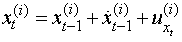
the weights are updated recursively using

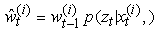where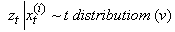

We evaluate this distribution at time for the parameters estimation by using the EM algorithm and SMC, and then calculate the output:

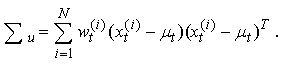
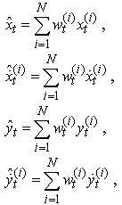The mean estimate of the target state and the covariance matrix of the estimate error are approximated by

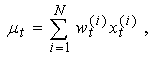
4. Experiment Results - Tracking Performance

An in-depth analysis of the tracking performance for the BOT problem is investigated in various works including Gordon et al., (1993) and Doucet et al., (2001). A bearings-only tracking problem is simulated to present implementation of the SMCEM algorithm based on both the mixture of Gaussians model of Kim and Stoffer (2008) and the Student’s-t. A target trajectory and associated measurements is generated according to equations (5) and (6) with the parameter values

,

the initial state of the target

and covariance .

The time between successive measurements is and a single bearing measurement is obtained in each time step.

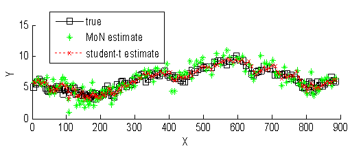Figure 2. Three scenarios for the BOT. Representation of the trajectories of the true target path (shown by a square), MoN (shown by an asterisk) and the Student’s-t estimate

Evaluation Statistic-Distribution comparison on technique based on the Normal mixture and Student’s-t

Figure 2 gives the true target path in the plane, with the position of the target at each time being shown by a square and the mixture of normal by an asterisk. The result of applying the SMCEM with particles is shown in the figure. The number of particles was chosen such that further increase in does not bring a significant improvement in the tracking performance. The cross symbol gives the Student’s-t estimate such that the estimate moves towards the true target path.

The performance is evaluated using the mean square error (MSE) and chi-square criterion Gallant and Long (1997) for each time. According to Sanjeev et al., (2004)

(7)

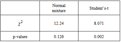
where denotes the estimate at time is the total number of realizations over which the MSE is averaged. Each of these realizations used observations from the same generated true state. Obviously, with increasing particles, the performance in terms of mean square error (MSE) improves. The MSE value (7.2197 and 11.0112 for mixture normal and Student’s-t) is obtained independently for each element of the state in the BOT problem. For the Student’s-t based filter, no tracks diverged. It can be seen that the accuracy of the position estimation of the Student’s-t particle filter is significantly higher than that of the normal mixture. Furthermore, our empirical implementation based on chi-square criterion, [Gallant and Long (1997), [see table] reveals that the technique based on the Student’s-t is statistically significant at 1% significance level.

4.1. Dynamic Modeling of a Vehicle Tracking

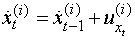
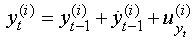
The proposed estimation technique was also applied to the problem of tracking a moving vehicle. Data were taken from the digital GSM real-time data logging tracking system, (see www.trackingtheworld.com). It models the dynamic properties of the tracked vehicle and estimates it using the proposed technique.

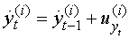
From the data collected, we estimate the vehicle’s position at time , and its velocity . Also at each time step we obtain a new measurement . the velocity evolves over time according to

.

The vehicle moves based on the evolved velocity according to a dynamics model:

.

The measurements are governed by a measurement model:

.

The measurement likelihood factor is

.

At each time step , we produce an estimate of the proposed technique about the tracked vehicle trajectory and velocity based on a set of measurements:

(8)

Equation (8) encodes the vehicle motion and is approximated using the Student’s-t distribution. The motion update of the particle filter is carried out using the vehicle dynamic model. The measurement update is carried out by computing the importance weights for all particles:

where .

The results for this case are presented in Figure 3. The Student’s-t based SMCEM algorithm is able to track the true path of the vehicle being tracked and remains stable and converges, showing that increasing the information provided by the measurements improves the accuracy and convergence of the estimation.

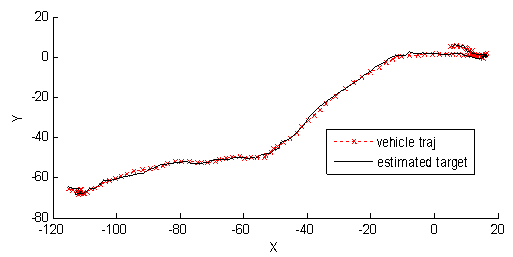Figure 3. Estimates of the vehicle being tracked

5. Conclusions

It has been shown in this paper that a Student’s-t distribution based particle filter provides a much better performance than the normal mixture based particle filter. An EM-type algorithm for solving a joint estimation-identification problem for nonlinear non-Gaussian state-space estimation when the observation model is uncertain is proposed. The expectation (E) step is implemented by the particle filter. Within this step, the distribution of states given the measurements as well as the state vectors is estimated. Consequently, in the maximization (M) step, the nonlinear measurement process parameters are approximated as a mixture of Normal model and as a Student’s-t model. The SMCEM algorithm based on both the mixture of Gaussians model of Kim and Stoffer (2008) and the Student-t is used to solve a nonlinear bearing-only tracking problem. It is shown that the accuracy of the position estimation of the Student’s-t filter is significantly higher than that of the normal mixture. Additionally, the method is applied to real life data taken from the digital GSM real-time data logging tracking system. It is again shown that the Student’s-t based algorithm is successful in accommodating nonlinear model for a target tracking scenario.