-
Paper Information
- Previous Paper
- Paper Submission
-
Journal Information
- About This Journal
- Editorial Board
- Current Issue
- Archive
- Author Guidelines
- Contact Us
International Journal of Probability and Statistics
p-ISSN: 2168-4871 e-ISSN: 2168-4863
2014; 3(1): 15-22
doi:10.5923/j.ijps.20140301.03
Small Area Estimation with Application to Disease Mapping
 Abstract
 Reference
 Full-Text PDF
 Full-text HTML
E. P. Clement
Department of Mathematics and Statistic University of Uyo, Uyo, Nigeria
Correspondence to: E. P. Clement, Department of Mathematics and Statistic University of Uyo, Uyo, Nigeria.
| Email: |  |
Copyright © 2012 Scientific & Academic Publishing. All Rights Reserved.
Small Area Estimation is important in survey analysis when domain (subpopulation) sample sizes are too small to provide adequate precision for direct domain estimators. Small Area Estimation (SAE) is a mathematical technique for extracting more detailed information from existing data sources by statistical modeling. The estimates are often mapped, so the technique is often generically called mapping. These maps and estimates (together with estimates of accuracy) are key information in aid allocation within a country. They are also increasingly important inputs to negotiations on allocation of international aid to particular countries. This paper provides a critical review of the main advances in small area estimation (SAE) methods in recent years with application to disease mapping. The review discusses in detail earlier developments of small area estimation methods in the field of disease mapping which serve as a necessary background for the new studies in disease mapping of small areas which we termed “Extensions”. Illustrative examples of the application of Small Area Estimation (SAE) to disease mapping are presented.
Keywords: Disease Mapping, Empirical Bayes (EB), Hierarchical Bayes (HB), Relative Risk (RR), Small Area Estimation (SAE), Standardized Mortality Ratios (SMRs)
Cite this paper: E. P. Clement, Small Area Estimation with Application to Disease Mapping, International Journal of Probability and Statistics , Vol. 3 No. 1, 2014, pp. 15-22. doi: 10.5923/j.ijps.20140301.03.
Article Outline
1. Introduction
- As with the analysis of any data set, it is always good practice to begin by producing and inspecting graphs. A feel for the data can then be obtained and any outstanding features identified. In spatial epidemiology this is called disease mapping.Disease mapping is considered as exploratory analysis used to get an impression of the geographical or spatial distribution of disease or the corresponding risk. Disease mapping is an epidemiological technique used to describe the geographic variation of disease and to generate etiological hypotheses about the possible causes for apparent differences in risks. A disease map is used for reporting the results of a geographical correlation study or to highlight geographical areas with high and low incidence, prevalence and mortality rates of specific disease and the variability of such rates over a spatial domain (small area). They can also be used to detect spatial clusters which may be due to common environmental, demographical, or cultural effects shared by neighbouring regions. The correct geographical allocation of health care resources would be greatly enhanced by the development of statistical models that allow a more accurate depiction of “true” disease occurrence and prevalence.The Millennium Development Goals (MDGs) provide a context for small area estimation, since local estimates (small area estimates) of disease rates and their updates have potential to provide fine-detailed national monitoring information against which progress can be measured. Small Area Estimation is a statistical technique involving the estimation of parameters for small sub-populations (small areas) where a sample has insufficient or no sample for the sub-population (small area) to be able to make accurate estimates for them. The term “small area” may refer strictly to a small geographical area such as a county, but may also refer to a “small domain”, that is, a particular demographic within an area. Small area estimation methods use models and additional data sources (such as census data) that exist for these small areas in order to improve estimates’ for them.Small area estimation is important in survey analysis when domain (sub-population or small area) sample sizes are too small to provide adequate precision for direct domain estimators. It is a mathematical technique for extracting more detailed information from existing data sources by statistical modeling. The estimates are often mapped to obtain and identify any outstanding features, so the technique is often generically called mapping. These maps and estimates (together with estimates of accuracy) are key information in aid allocation within a country. They are also increasingly important inputs to negotiations on allocation of international aid to particular countries by the World Health Organization (WHO) and other International Aid Agencies (IAA).The purpose of this paper is to provide a critical review of the main advances in small area estimation with application to Health surveys in general and disease mapping in particular. Four statistical models: Poisson-gamma, log-normal, conditional autoregression normal (CAR-normal) and two-level models are discussed. The empirical bayes (EB) and the hierarchical bayes (HB) models are also discussed as extensions to the four basic models. The review discusses in detail earlier developments of small area estimation (SAE) methods in the field of disease mapping which serve as a necessary background for the various extensions of the disease mapping models proposed in recent literature. Illustrative examples of studies so far proposed are presented. The paper ends with a brief summary and some concluding remarks.
2. Application of Small Area Estimation to Health
- Small area estimation of health related characteristics has attracted a lot of attention in the Western countries like the U.S, Britain, U. K and Canada because of a continuing need to assess health status, health practices and health resources at both the national and sub-national levels. Reliable estimates of health-related characteristics help in evaluating the demand for health care and the access individuals have to it. Health care planning often takes place at the state and sub-state levels because health characteristics are known to vary geographically.Health System Agencies in the United States, mandated by the National Health Planning Resource Development Act of 1994, are required to collect and analyse data related to the health status of the residents and to the health delivery systems in their health service area[1].The U.S. National Centre for Health Statistics pioneered the use of synthetic estimation, based on implicit linking models, developing state estimates of disability and other health characteristics for different groups from the National Health Interview Survey (NHIS)[2].[3] studied HB estimation of overweight prevalence for adults by states, using data from NHANES III,[4] produced survey-weighted HB estimates of small area prevalence rates for states and age groups, for up to 20 binary variables related to drug use, using data from pooled National Household Surveys on Drug Abuse.[5] studied EB estimates of state-wide prevalence of the use of alcohol and drugs (e.g. Marijuana) among civilian non-institutionalized adults and adolescents in the United States. These estimates are used for planning and resource allocation, and to project the treatment needs of dependent users.Direct (or crude) estimates of rates, called standardized mortality ratios (SMRs) can be very unreliable, and a map of crude rates can badly distort the geographical distribution of disease incidence or mortality because the map tends to be dominated by areas of low population. Disease mapping, using model-based estimators, has received increased attention in recent years. Typically, sampling is not involved in disease mapping applications.
3. Mortality and Disease Rates Models
- Mortality and disease rates of small area in a region or a county are often used to construct disease maps such as cancer atlases. Such maps are used to display geographical variability of a disease and identify high-rate areas warranting intervention. A simple small area model is obtained by assuming that the observed small area counts
 are independent Poisson variables with conditional mean
 | (1) |
 .where
  is the true rate,
  is the number exposed in the ith area, and
  are the scale and shape parameters of the gamma distribution under this model, smoothed estimates of
  are obtained using EB or HB methods[6],[7].If
  denotes a set of “neighbouring” areas of the ith area, then a conditional autoregression (CAR) spatial model assumes that the conditional distribution of
  given
given  is given by
  | (2) |
 are known constants satisfying
  and
and  is the unknown parameter vector.CAR spatial models of the form (2) on log rates
 | (3) |
 can be extended to incorporate area level covariates
  for example:
 | (4) |
 | (5) |
 can also be modeled if
  are asummed independently distributed conditional on
  and
and | (6) |
 are assumed to be conditionally independent Poisson variables with
  | (7) |
 where
where  and
and  denote the number of deaths due to a disease (say malaria) and the population at risk at site (or area) 1 respectively and
  and
and  denote the number of deaths due to the same disease and the population at risk at site (or area) 2 respectively.[9] showed that the bivariate model leads to improved estimates of the rate
  compared to estimates based on separate univariate models.
4. Disease Mapping
- Mapping of small area mortality (or incidence) rates of disease such as cancer, malaria is a widely used tool in Public Health research. Such maps permit the analysis of geographical variation in rates of diseases which may be useful in formulating and assessing etiological hypotheses, resource allocation, and identifying areas of unusually high risk warranting intervention.The following are examples of studies of disease rates in the literature:[6] studied lip cancer rates in the 56 counties (small areas) of Scotland;[7] studied the incidence of leukemia in 281 census tracts (small areas) of upstate, New York.[8] studied all cancer mortality rates for white males in health service areas (small areas) of the United States;[10] studied prostrate cancer rates in Scottish counties; and[11] studied infant mortality rates for local health areas (small areas) in British Columbia, Canada.Worthy of note is the fact that sampling is not used in disease mapping only administrative data on event counts and related auxiliary variables are used in disease mapping.
4.1. Disease Mapping Models
- Suppose that the country (or the region) used for disease mapping is divided into m non-overlapping small areas. Let
 be the unknown relative risk (RR) in the ith area. A direct (or crude) estimator of
  is given by the standardized mortality ratio (SMR)
 | (8) |
 and
and  denote the observed and expected number of deaths (cases) over a given period
  respectively.Where:
 | (9) |
 as parameters instead of relative risks, and a crude estimator of
  is then given by
  . However, the two approaches are equivalent since
  is treated as a constant.A common assumption in disease mapping is that
  Poisson
  . Under this assumption, the maximum likelihood (ML) estimator of
  is the SMR,
  .However, a map of crude rates
  can badly distort the geographical distribution of disease incidence or mortality because it tends to be dominated by areas of low population,
  exhibiting extreme SMR’s that are least reliable.
 | (10) |
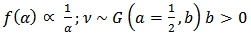
4.1.1. Poisson-Gamma Model
- Given a two-stage model, at the first stage, assume
 Poisson
  ,
,  = 1, 2,…, m. A conjugate model linking the relative risks
  is assumed in the second stage:
  gamma
gamma  denotes the gamma distribution with shape parameter
  and scale parameter
  . Then we have
 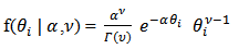 | (11) |
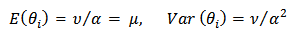 | (12) |
 , the bayes estimators of
  and posterior variance of
  are obtained from (3) by changing
  to
to  and
and  to
to  such that:
 | (13) |
 | (14) |
 and
and  from the marginal distribution,
  negative binomial, using the log likelihood is:
 | (15) |
 and
and  do not exist. However,[12] obtained simple moment estimators by equating the weighted sample mean
 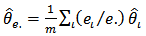 and the weighted sample variance
  to their expected values and then solving the resulting moment equations for
  and
and  , where
  . This leads to moment estimators,
  and
and  , given by:
 | (16) |
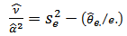 | (17) |
 and
and  into (13) we get the empirical Bayes (EB) estimator of
  as
as 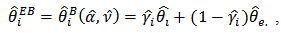 | (18) |
 . It should be noted that
  is a weighted average of the direct estimator (SMR)
  and the synthetic estimator
  , and more weight is given to
  as the area expected deaths,
  , increase. If
 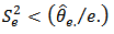 then
then  is taken as the synthetic estimator
  . The empirical bayes (EB) estimator is nearly unbiased for
  in the sense that its bias is of order
  , for large
  . The Jackknife method may be used to obtain a nearly unbiased estimator of MSE
  . The jackknife estimator is given by
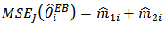 | (19) |

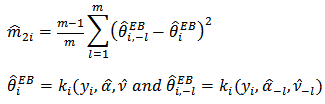 where
where  are the delete
  moment estimators obtained from
  . Note that
  is area-specific in the sense that it depends on
  .[13] obtained a Taylor expansion estimator of MSE, using a parametric bootstrap to estimate the covariance matrix of
  .The linking gamma model on the
  can be extended to allow for area -level covariates
  , such as degree of relative risk
  .[6] allowed varying scale parameters,
  , and assumed a loglinear model on
 | (20) |
 | (21) |
 | (22) |
 . The posterior mean approximation is used as the empirical bayes (EB) estimator and the posterior variance approximation as a measure of its variability. (a) Hierarchical Bayes (HB) Estimation Let
  respectively denote the relative risk (RR), observed and expected number of cases (deaths) over a given period in the ith area
  . A hierarchical bayes (HB) estimation of the Poisson-gamma model, is given by:
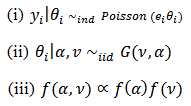 | (23) |
 See[7].The joint posterior
  is proper if at least one
  is greater than zero. The Gibbs conditionals are given by:
  | (24) |
 posterior quantities of interest may be computed, in particular, the posterior mean
  and posterior variance
  for each area
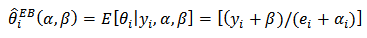
4.1.2. Log-Normal Model
- Log-normal two-stage models have also been proposed. The first-stage model is not changed, but the second-stage linking model is changed to

 As in the case of logit-normal models, implementation of empirical bayes (EB) is more complicated for the log-normal model because no closed-form expression for the bayes estimator,
  and the posterior variance,
  exist.[6] approximated the posterior density,
  by a multivariate normal which gives an explicit approximation to
  and
and Maximum likelihood estimators of model parameters
 were obtained using the EM algorithm and then used in the approximate formula for
  to get EB estimators
  The empirical bayes (EB) estimator
  however, is not nearly unbiased for
  Moment estimators of
  proposed by[15] may be used to simplify the calculation of Jackknife estimator of
 The basic log-normal model readily extends to the case of covariates
 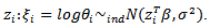 (a) Hierarchical Bayes Estimation A hierarchical bayes (HB) estimator of the basic log-normal model is given by:
  | (25) |
 The joint posterior
  is proper if at least one
  is greater than zero, it is easy according to[2] to verify that the Gibbs conditionals are given by:
 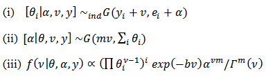 | (26) |
 Where
Where  and
and  with
with  We can use
  to draw the candidate,
  noting that
  and
and 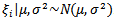 . The acceptance probability used in the M-H algorithm is then given by
  . The basic log-normal model with Poisson counts
  as noted earlier, readily extends to the case of covariates
  where (ii) and (iii) of (25) become respectively:
  | (27) |
4.1.3. Car-Normal Model
- The basic log-normal can be extended to allow spatial correlations; mortality data sets often exhibit significant spatial relationship between the log relative risks,

 A simple conditional autoregression (CAR)-normal model on
  assumes that
  is a multivariate normal specified by:
 | (28) |
 | (29) |
 is the correlation parameter and
  is the “adjacency” matrix of the map given by
  are adjacent areas and
  otherwise. It follows from[17] that
  is multivariate normal with mean
  and covariance matrix
 where
where  is bounded above by the inverse of the largest eigenvalue of
 .[6] approximated the posterior density,
  similar to the log-normal case. The assumption of equation (29) of a constant conditional variance for the
  results in the conditional mean of (28) proportional to the sum of the neighbouring
  rather than the mean of the neighbouring
  (local mean).[18] Proposed an alternative joint density of the
  given by:
 | (30) |
 | (31) |
 | (32) |
 the number of neighbours of area
  and the conditional mean is equal to the mean of the neighbouring values
 In the context of disease mapping, the alternative specification may be more appropriate[2].(a) Hierarchical Bayes Estimation As noted earlier, the basic log-normal can be extended to allow spatial covariates. A hierarchical bayes (HB) estimator of the spatial CAR-normal model is given by:
  | (33) |
 where
where  denotes the maximum value of
  in the CAR-model, and
  is the “adjacency” matrix of the map with
  are adjacent areas and
  otherwise. [16] obtained the Gibbs conditionals. In particular,
  and
and  does not admit a closed form in the sense that the conditional is known only up to a multiplicative constant. Monte Carlo Markov Chain (MCMC) samples can be generated directly from the three conditionals, but we need to use the M-H algorithm to generate samples from the conditionals
  [2].
[2].4.2. Two-Level Models
- Let
 denote the number of cases (deaths) and the population at risk in the
  age class in the
  area
area  respectively. Using the data
  it is of interest to estimate the age-specific mortality rates
  and the age-adjusted rates
  where the
  are specified constant. The basic assumption is
  | (34) |
 | (35) |
 | (36) |
 | (37) |
 vector of covariance and
  is an “offset” corresponding to age class
  . [1] assumed that flat prior
  and proper diffuse (that is, proper with very large variance) priors for
  For model selection, they used the posterior expected predictive deviance, the posterior predictive value and measures based on the cross-validation productive densities.
5. Examples
- We now present some illustrative examples of the application of Small Area Estimation (SAE) in health – disease mapping.(i) Lip Cancer[16] modeled
 He also considered a CAR spatial model on the
  which relates each
  to a set of neighbourhood areas of area
  He developed model-based estimates of lip cancer incidence in Scotland for each of 56 counties. [6] applied empirical bayes (EB) estimation to data on observed cases,
  and expected cases,
  of lip cancer registered during the period 1975 – 1980 in each of 56 counties (small area) of Scotland. They reported the SMR, the empirical bayes (EB) estimate of
  based on the Poisson-gamma model
  and the approximate empirical bayes (EB) estimates of
  based on the log-normal model and the CAR-normal model (denoted
 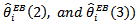 for each of the 56 counties (all values multiplied by 100). The SMR-values varied between 0 and 652 while the empirical bayes (EB) estimates showed considerably less variability across counties as expected:
  varied between 31 and 422 (with cv = 0.78) and
  varied between 34 to 495 (with cv=0.85), suggesting little difference between the two sets of empirical bayes (EB) estimates. Ranks of empirical bayes (EB) estimates differed little from the corresponding ranks of the SMRs for most counties, despite less variability exhibited by the empirical bayes (EB) estimates. For the CAR-normal model, the adjacency matrix, Q, was specified by listing adjacent counties for each county
 The maximum likelihood (ML) estimates of
  was 0.174 compared to the upper bound of 1.175, suggesting a high degree of spatial relationship in the data set. Most of the CAR estimates,
  differed little from the corresponding estimates
 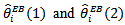 based on the independence assumption. Counties with few cases,
  and SMRs differing appreciably from adjacent counties are the only counties affected substantially by spatial correlation. For instance, county number 24 with
  is adjacent to several low-risk counties, and the CAR estimate
  is substantially smaller than
  and
and  based on the independence assumption. [16] applied hierarchical bayes (HB) estimator to the same data using the log-normal and the CAR-normal models. The hierarchical bayes (HB) estimates
  of lip cancer incidence are very similar for the two models, but the standard errors,
  are smaller for the CAR-normal as it exploits the spatial structure of the data. [19] proposed a spatial log-normal model that allows covariates
 It is given by:
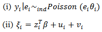 | (38) |
 does not include an intercept term.
  have joint density of (30):
 , where
  for all
 (iii)
(iii)  and
and  are mutually independents with
 | (39) |
 admit closed forms. They also established conditionals for the propriety of the joint posterior, in particular, we need
  (ii) Leukemia Incidence [19] applied the HB method based on the model given in (39), to leukemia incidence estimation for m=281 census tracts (small area) in an eight-county region of upstate New York. Here
  are neighbours and
  otherwise, and
  is a scalar
  variable
  denoting the inverse distance of the centroid of the ith census tract from the nearest hazardous waste site containing trichloroethylene (TCE), a common contaminant of ground water (See[19] for details).(iii) Mortality Rates [8] applied the hierarchical bayes (HB) method to estimate age-specific and age-adjusted mortality rates for U.S. Health Service Areas (HSAs). They studied one of the disease categories, all cancer for white males, presented in the 1996 Atlas of United States Mortality. The number of HSAs (small areas), m, is 789 and the number of age categories, J, is 10:0-4, 5-14, …, 75 – 84, 85 and higher, coded as 0.25, 1, …,9. The vector of auxiliary variables is given by
 for
for  and
and  where the value of the “knot” was obtained by maximizing the likelihood based on marginal deaths
  and population at risk,
  , where
  with
with  . The auxiliary vector
  was used in the Atlas model based on a normal approximation to
  with mean
  and matching linking model given by (36) where
  is the crude rate. [8] used unmatched sampling linking model, based on the Poisson sampling model of (34) and the linking models of (35) – (37). We denote these models as models 1,2 and 3 respectively. Also they used the Monte Carlo Markov Chain (MCMC) samples of generated from the three models to calculate the values of the posterior expected predictive deviance.
  using the chi-square measure
  They also calculated the posterior predictive p-values, using
  the standardized cross-validation residuals
  | (40) |
 denotes all elements of
  except
  (See[2]; section 10.2.28). The residuals
  were summarized by counting:(a) the number of
  such that
  called “outliers” , and (b) the number of HSAs is such that
  for at least one
 called
  of HSAs”.[20] used models and methods similar to those in[19] to estimate age-specific and age-adjusted mortality rates for chronic obstructive pulmonary disease for white males in HSAs.
 6. Extensions
- Various extensions of the disease mapping models, studied so far have been proposed in recent literature.[9] proposed a two-stage, bivariate logit-normal model to study joint relative risks (or mortality rates),
 of two cancer sites (e.g. lung and large bowel cancers) or two groups (e.g. lung cancer in males and females) over several geographical areas. Denote the observed and expected number of deaths at the two sites as
  respectively for the ith area
  The first stage assumes that
 , where * denotes that
 The joint risks
  are linked in the second stage by assuming that
  bivariate normal with means
  standard deviations
  and correlation
  denoted
  Bayes estimators of
  and
and  involve double integrals which may be calculated numerically using Gauss-Hermite quadrature. Empirical bayes (EB) estimators are obtained by substituting maximum likelihood (ML) estimators of model parameters in the bayes estimators.[9] applied the bivariate empirical bayes (EB) method to two data sets consisting of cancer mortality rates in 115 counties of the State of Missouri during 1972 – 1981. (i) Lung and large bowel cancers (ii) Lung cancer in males and females The empirical bayes (EB) estimates based on the bivariate model lead to improved efficiency for each site (group) compared to the empirical bayes (EB) estimates based on the univariate logit-normal model, because of significant correlation:
  for data set (i) and
  for data set (ii).[21] first-order approximation to the posterior variance was used as a measure of variability of the empirical bayes (EB) estimates. [22] extended the bivariate model by introducing spatial correlations (via CAR) and covariates into the model. They used a hierarchical bayes (HB) approach instead of the empirical bayes (EB) approach. They applied the bivariate spatial model to male and female lung cancer mortality in the State of Missouri, and constructed disease maps of male and female lung cancer mortality rates by age group and time period. [11] extended the Poisson-gamma model to handle nested data structures, such as a hierarchical health administrative structure consisting of local health districts,
  in the first level and local health areas,
  within districts in the second level
  The data consist of incidence or mortality counts
  and the corresponding population at risk counts,
  [11] derived empirical bayes (EB) estimates of the local health area rates
  using a nested error Poisson-gamma model. The bayes estimator of
  is a weighted combination of the crude local area rate,
  the correspond crude district rate,
  and the overall rate
  where
where  and
and  and
and  similarly defined. [11] used the[21] first-order approximation to posterior variance as a measure of variability. They applied the nested error model to infant mortality data from the province of British Columbia, Canada.
 7. Concluding Remarks
- Small area estimation of health related characteristics has attracted a lot of attention in the Western countries like the U.S., U.K., and Canada because of a continuing need to assess health status, health practices and health resources at both the national and sub national levels. Reliable estimates of health related characteristics help in evaluating the demand for health care and the access individuals have to it. Mortality and disease rates of small area in a region or a county are often used to construct disease maps which are used to display geographical variability of a disease and identify high rate and, or high risk areas warranting interventions. This article attempts to overview the main advances in small area estimation methods in the field of disease mapping and some relevant statistical models in disease mapping. A critical review of earlier developments of small area estimation methods in the field of disease mapping which serve as a necessary background for the various extensions of disease mapping models proposed in recent literature with illustrative examples are presented. Two important issues not considered are model selection and model diagnostics. As mentioned earlier; small area estimation is one of the few fields in survey sampling, where it is widely recognized that the use of model dependent is often inevitable. Given the growing use of small area estimates and their immense importance, it is imperative to develop efficient tools for the selection of their goodness of fit. A further issue which certainly deserves consideration is the objective comparison of the different statistical models for disease mapping and an evaluation of the quality of their forecasts. These will be our focus in a forthcoming article.