Onyeka-Ubaka J. N.1, Abass O.2, Okafor R. O.1
1Department of Mathematics, University of Lagos, Akoka, Lagos, +234, Nigeria
2Department of Computer Science, University of Lagos, Akoka, Lagos, +234, Nigeria
Correspondence to: Onyeka-Ubaka J. N., Department of Mathematics, University of Lagos, Akoka, Lagos, +234, Nigeria.
| Email: |  |
Copyright © 2012 Scientific & Academic Publishing. All Rights Reserved.
Abstract
The parameters  and
and  are restricted to be non-negative in GARCH model, which have some consequences for the stationarity condition, and although the disturbances
  have mean 0, they are clearly not white noise because of their time-varying asymmetric probability density functions. Thus, this stationary process is capable of capturing well known phenomena present in financial markets such as volatility clustering, marginal distributions having heavy tails and thin centres (Leptokurtosis); return series appearing to be almost uncorrelated over time but to be dependent through higher moments. The possibility of having dependence between higher conditional moments, most notably variances, involves examining nonlinear stochastic processes from a more realistic perspective in time series data. This motivates the consideration of nonlinear models. The results obtained through Monte Carlo simulations established the practicability and small sample performance of symmetric models under Gaussian distributions. The results also showed that the corresponding standard errors are very small indicating that estimators are asymptotically unbiased, efficient and consistent at least within the sample.
Keywords:
GARCH, Symmetric, Simulation, Conditional Variance, Stationarity
Cite this paper: Onyeka-Ubaka J. N., Abass O., Okafor R. O., Conditional Variance Parameters in Symmetric Models, International Journal of Probability and Statistics , Vol. 3 No. 1, 2014, pp. 1-7. doi: 10.5923/j.ijps.20140301.01.
1. Introduction
Financial time series present various forms of non linear dynamics, the crucial one being the strong dependence of the variability of the series on its own past and furthermore, with the fitting of the standard linear models being poor in these series. The autoregressive conditional heteroskedasticity (ARCH) model has become one of the most important models in financial applications. These models are non-constant variances conditioned on the past, which are a linear function on recent past disturbances Onyeka-Ubaka and Abass[9] and Dallah, Okafor and Abass[5]. This means that the more recent news will be the fundamental information that is relevant for modelling the present volatility. Moreover, the accuracy of the forecast over time improves when some additional information from the past is considered. Specifically, the conditional variance of the innovations will be used to calculate the percentile of the forecasting intervals, instead of the homoskedastic formula used in standard time series models. Recent developments in economic and financial econometrics suggest the use of nonlinear time series structures to model the attitude of investors toward risk and expected returns. This is because the conditional variance is not constant over time. Hence, this paper, therefore, is set out to establish the practicability and small sample performance of Generalized Autoregressive ConditionalHeteroskedasticity (GARCH) model within the Gaussian framework.
2. Literature Review
Empirical studies show that models which present some nonlinearity can be modelled by conditional specifications, in both conditional mean and variance. A stochastic process  is a model that describes the probability structure of a sequence of observations over time Zhu[13]. A time series
  is a sample realization of a stochastic process that is observed only for a finite number of periods, indexed by
  Onyeka-Ubaka[8]. Any stochastic process can be partially characterized by the first and second moments of the joint probability distribution: the set of means,
  and the set of variances and covariances
 . In order to get consistent forecast methods, we need that the underlying probabilistic structure would be stable over time. So a stochastic process is called weak stationary or covariance stationary when the mean, the variance and the covariance structure of the process is stable over time, that is:
 Let
Let  refer to the univariate discrete time-valued stochastic process to be predicted (e.g. the rate of return of a particular stock or market portfolio from time t -1 to t) where
  is a vector of unknown parameters and
  denotes the conditional mean given the information set
  available in time t -1. The innovation process for the conditional mean,
  , is then given by
  with corresponding unconditional variance
  , zero unconditional mean and
  ,
, 
 . The conditional variance of the process given by
  is defined by
  . Since investors would know the information set
  when they make their investment decisions at time t -1, the relevant expected return to the investors and volatility are
  and
and  , respectively.An ARCH process,
  , can be presented as:
 | (1) |

 | (2) |
where 
 ,
,  is a time-varying positive and measurable function of the information set at time t -1,
  is a vector of predetermined variables included in
  , g(.) is a linear or nonlinear functional form. By definition,
  is serially uncorrelated with mean zero, but a time varying conditional variance equal to
  . The conditional variance is a linear or nonlinear function of lagged values of
  and
and  , and predetermined variables
  included in
  . In the sequel, for notational convenience, no explicit indication of the dependence on the vector of parameters,
  , is given when obvious from the context. Since very few financial time series have a constant conditional mean zero, an ARCH model can be presented in a regression form by letting
  be the innovation process in a linear regression:
 | (3) |
 where
where  is a
is a  vector of endogenous explanatory variables included in the information set
  , b is a
  vector of unknown parameters,
  is the random disturbance term, and the subscript t indicates that
  and
and  are series of equally spaced observations through time. The use of the time series regression model underlies a number of assumptions concerning the form of the model, the independent variable and the disturbance terms. Provided that these assumptions hold: (i) Zero mean: E[
 ] = 0(ii) Constant Variance: E[
 ] =
] =  (iii) Non-autoregression: E[
 ] = 0 (
 )It is possible to estimate optimally the regression parameters and their variances with the following formulas:
 | (4) |
 | (5) |
 | (6) |
 | (7) |
 .where
 | (8) |
The estimators are optimal in the sense that they are unbiased, efficient and consistent. Unbiased estimators are those in which the expected value of the estimator, say  , is equal to the true value, b. An estimator is relatively efficient if it has a smaller variance than any other estimator of b, and it will be consistent if both its bias and variance approach zero as the sample size approaches infinity. Together these properties mean that an estimator will be centered around the true value as the sample size increases. Of particular interest are assumptions (i) and (iii), which, together, imply that the covariance of any two disturbance terms (i. e.,
  ) is equal to zero. This can be seen as follows:
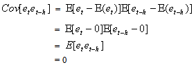 This means that one assumes that disturbances at one point in time are not correlated with any other disturbances. The basic indicator of whether the non-autoregression assumption is violated is whether there is a sample correlation between the various random disturbance terms. To obtain a visual indication of the nature of the correlation, it is helpful to construct a correlogram that provides a graphical representation of the estimated autocorrelation function with time lags and autocorrelation coefficients forming the axes. The paper observes that the main problem with an ARCH model of Engle[6] in empirical application is that it requires a large number of lags to catch the nature of the volatility; this can be problematic as it is difficult to decide how many lags to include and produces a non-parsimonious model where the non-negativity constraint could be failed. To facilitate the computational problems of ARCH model, Bollerslev[1] proposed a generalization of the ARCH (q) process to allow for past conditional variances in the current equation.
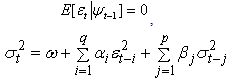 | (9) |
where These conditions on parameters ensure strong positivity of the conditional variance (9). If the study writes the equation (9) in terms of lag-operator B, it gets
 | (10) |
where and
and | (11) |
The model is covariance stationary if all the roots of  lie outside the unit circle, or equivalently if
  . That is, if

 Then, its long-run average variance (unconditional variance) is equal to
  | (12) |
This model differs to the ARCH model in that it incorporates squared conditional variance terms as additional explanatory variables. This allows the conditional variance to follow an ARMA process in the squared innovations of orders max(p, q) and p,[ARMA(max(p, q), p)], respectively: | (13) |
The GARCH model is usually much more parsimonious and often a GARCH (1, 1) model is sufficient, this is because the GARCH model incorporates much of the information that a much larger ARCH model with large number of lags would contain.
3. Methodology
In this paper, the modelling is proceeded by specifying and estimating a model and then checking its adequacy. If model defects are detected at the latter stage, model revisions are made until a satisfactory model has been found. Then the model may be used for forecasting. Figure 1 depicts the main steps of a GARCH analysis and it is on these steps that this research is organized accordingly.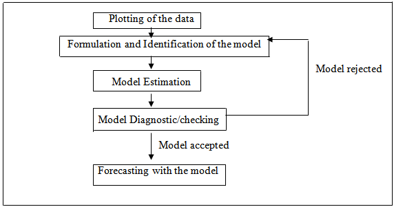 | Figure 1. GARCH analysis (figure adapted from Box-Jenkins (1976) step by step approach) |
4. Results and Discussion
The estimation of GARCH model involves the maximization of a likelihood function constructed under the auxiliary assumption of an independent identically distributed (i.i.d.) distribution for the standardized innovation  Let
Let  denote the density function for
  =
=  , with mean zero and variance one, where
  is the nuisance parameter,
  is the vector of the parameter of f to be estimated. To implement the maximum likelihood procedure, we use normal, the most commonly distribution in the literature.
 | (14) |
Since the normal distribution is uniquely determined by its first two moments, only the conditional mean and variance parameters enter the log-likelihood function in (9) i.e.  The log-likelihood is
 It follows that the score vector
  takes the form:
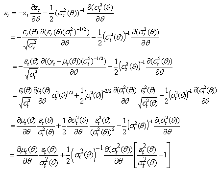 | (15) |
When  where
where  are the conditional mean parameters and
  are the conditional variance parameters, the score takes the form:
 where
where 
Even in the case of the symmetric GARCH (p, q) with normally distributed innovations, we have to solve a set of  nonlinear equations in (9). Numerical techniques are used in order to estimate the vector of parameters
  . The problem faced in nonlinear estimation, as in the case of the GARCH models, is that there are no closed form solutions. So, an iterative method has to be applied to obtain a solution. Iterative optimization algorithms work by taking an initial set of values of the parameters, say
  , then performing calculations based on these values to obtain a better set of parameters values
  . The process is repeated until the likelihood function
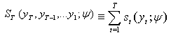 | (16) |
no longer improves between iterations. If  is a trial value of the estimate, then expanding
  and retaining only the first power of
  -
-  , we obtain
 .At the maximum,
  should equal zero. Rearranging terms, the correction for the initial value,
  , obtained is
 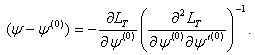 | (17) |
Let  denote the parameter estimates after the
  iteration. Based on (17) the Newton-Raphson algorithm computes
  as:
as: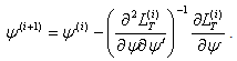 | (18) |
The scoring algorithm is a method closely related to the Newton-Raphson algorithm and was applied by Engle[6] to estimate the parameters of the ARCH (q) model. The difference between the Newton-Raphson method and the method of scoring is that the former depends on observed second derivatives, while the latter depends on the expected values of the second derivatives. So, the scoring algorithm computes  as:
as: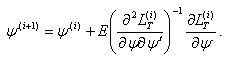 | (19) |
The assumption of normally distributed standardized innovations is often violated by the data. If the true distribution is instead leptokurtic, then the maximum is still consistent, but no longer efficient. In this case the maximum likelihood method is interpreted as the ‘Quasi-Maximum Likelihood (QML) method. Bollerslev and Wooldridge[3], based on Wesis[12] and Pagan and Sabau[10], showed that the maximization of the normal log-likelihood function can provide consistent estimates of the parameter vector  even when the distribution of
  in non-normal, provided that
  These estimates are, however, inefficient with the degree of inefficiency increasing with the degree of departure from normality Pagan and Schwert[11]. So, the standard errors of the parameters have to be adjusted. Let
  be the estimate that maximizes the normal log-likelihood function, in equation (16), based on the normal density function in (15) and let
  be the true value. Then, even when
  is non-normal, under certain regularity conditions: (
 Thus,
Thus,  is a maximum likelihood estimator based on a mis-specified model. Under regularity conditions, the QML estimator converges almost surely to the pseudo true value
 .For symmetric departures from normality, the quasi-maximum likelihood estimation is generally close to the exact maximum likelihood estimation (MLE). But, for non-symmetric distribution, Engle and Kroner[7] showed that the loss in efficiency may be quite high. The practical applicability and small sample performance of the MLE procedure for the GARCH process is studied by Monte Carlo simulations.
4.1. Monte Carlo Experiments
A hybrid Monte Carlo experiment was performed using the normal distribution as data generating processes by introducing an auxiliary vector to avoid random walk behaviour. The momentum samples are discarded after sampling. The end result of hybrid Monte Carlo experiment is that the proposals move across the sample space in large steps and are therefore less correlated and converge to the target distribution more rapidly. Through the Monte Carlo experiment, the model considered for  is a GARCH (1, 1) given by
 where
where  is a standard Normal random variable and n = 50, 60, 70, 80, 250, 700, 1000 and 3000. The conditional mean,
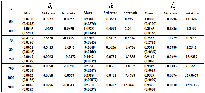
  , is assumed to follow an AR (1) model in the simulation experiment.Table 1 lists the Monte Carlo mean, standard error (Std error) and t-statistic for the parameter vector
  across M = 1000 Monte Carlo simulations. The simulation algorithm generates n + 1000 observations for each series, saving only the last n. This operation is performed in order to avoid dependence on initial values. The calculations were carried out in MATLAB (R2008b). For any set of parameter
  , the starting estimate for the variance of the first observation is often taken to be the observed variance of the residuals. It is easy to calculate the variance forecast for the second. The GARCH updating formula takes the weighted average of the unconditional variance, the squared residuals for the first observation and the starting variance and estimates of the second. This is input into the forecast of the third variance, and so forth. Ideally, this series is large when the residuals are large and small when they are small. The likelihood function provides a systematic way to adjust the parameters
  to give the best fit.
Table 1. Estimated Parameters (and the Estimated Standard Errors) for the Centered Normal GARCH (1, 1) Model
 |
| |
|
Inspection of Table 1 reveals that for all sample sizes, the averages obtained from the exact MLE are close to the true parameter values. The corresponding standard errors are very small indicating that estimators are asymptotically unbiased, efficient and consistent. The standard GARCH model has news impact curve, which is symmetric and centred at  . That is, positive and negative return shocks of the same magnitude produce the same amount of volatility. Also, larger return shocks forecast more volatility at a rate proportional to the square of the size of the return shock. If a negative return shock causes more volatility than a positive return shock of the same size, the GARCH model under predicts the amount of volatility following bad news and over predicts the amount of volatility following good news. Furthermore, if large return shocks cause more volatility than a quadratic function allows, then the standard GARCH model under predicts volatility after a large return shock and over predicts volatility after a small return shock.Table 1 summarizes the estimates coefficients from the GARCH (1, 1) model with the true value set of parameters
  = {-0.0016, 0.2510, 0.9895}, that is, the simulation model:
 . The P-values of the estimated parameters shown in the brackets are statistically significant with values almost less than 0.05. Where Std error is the Standard errors and t-statistic is T Statistics obtained by dividing the mean by the standard error. Monte Carlo simulations are computed 1000 replications. Each replication gives a sample size n = 50, 60, 70, 80, 250, 700, 1000 and 3000 observations.
5. Conclusions
The GARCH model is characterized by a symmetric response of current volatility to positive and negative lagged errors  , since
  is uncorrelated with its history. This could be interpreted conveniently as a measure of news entering a financial market at time t. The paper established that the GARCH (1, 1) model captures volatility clustering and leptokurtosis present in high frequency financial time series data. The Monte Carlo simulations showed the practicability and sample performance analysis of the GARCH (1, 1) model under normal distribution. The simulated results also showed that the corresponding standard errors are very small indicating that estimators are asymptotically unbiased, efficient and consistent. From the discussions, we observe that the simple structure of the model imposes important limitations on GARCH models. Thus:(i) GARCH models, however, assume that only the magnitude and not the positivity or negativity of unanticipated excess returns determines conditional variance
  . If the distribution of
  is symmetric, the change in variance tomorrow is conditionally uncorrelated with excess returns today.(ii) The GARCH models are not able to explain the observed covariance between
  and
and This is possible only if the conditional variance is expressed as an asymmetric function of
  (iii) GARCH models essentially specify the behaviour of the square of the data. In this case a few large observations can dominate the sample.(iv) The negative correlation between stock returns and changes in returns volatility, that is, volatility tends to rise in response to “bad news”, (excess returns lower than expected) and to fall in response to “good news” (excess returns higher than expected) are also observed. This limitation is called leverage effect and can be tackled with asymmetric models.
References
| [1] | Bollerslev, T. (1986). Generalized Autoregressive Conditional Heteroskedasticity, Journal of Econometrics, 31, 307-327. |
| [2] | Bollerslev, Engle and Wooldridge (1988). A Capital Asset Pricing Model with Time-Varying Covariances. Journal of Political Economy. 96, 116-131. |
| [3] | Bollerslev, T. and Wooldridge, J. M. (1992). Quasi- Maximum Likelihood Estimation and Inference in Dynamic Models with Time-Varying Covariances. Econometric Reviews, 11, 143-173. |
| [4] | Box, G.E.P. and Jenkins, G. W. (1976). Time Series Analysis: Forecasting and Control, Holden-Day, San Francisco. |
| [5] | Dallah, H., Okafor, R. O. and Abass, O. (2004). A Model-Based Bootstrap Method for Heteroskedasticity Regression Models. Journal of Scientific Research and Development, 9, 9 - 22. |
| [6] | Engle, R. F. (1982). Autoregressive Conditional Heteroskedasticity with Estimates of United Kingdom Inflation. Econometrica, 50, 987-1007. |
| [7] | Engle, R. F. and Kroner, K. F. (1995). Multivariate Simultaneous Generalized ARCH. Econometric Theory, 11, 122-150. |
| [8] | Onyeka-Ubaka, J. N. (2013). A Modified BL-GARCH Model for Distributions with Heavy Tails. A Ph.D Thesis, University of Lagos, Akoka, Nigeria. |
| [9] | Onyeka-Ubaka, J. N. and Abass, O. (2013). Central Bank of Nigeria (CBN) Intervention and the Future of Stocks in the Banking Sector. American Journal of Mathematics and Statistics,3(6): 407-416. |
| [10] | Pagan, A. R. and Sabau, H. (1987). On the Inconsistency of the MLE in Certain Heteroskedastic Regression Models, University of Rochester, Department of Economics, Mimeo. |
| [11] | Pagan, A. R. and Schwert, G. W. (1990). Alternative Models for Conditional Stock Volatility, Journal of Economics, 45, 267-290. |
| [12] | Weiss, A. (1986). Asymptotic Theory for ARCH Models: Estimation and Testing. Econometric Theory, 2, 107-131. |
| [13] | Zhu, F. (2011). A negative binomial integer-valued GARCH model. Journal of Time Series Analysis, 32, 54-67. |
 Abstract
 Reference
 Full-Text PDF
 Full-text HTML