-
Paper Information
- Paper Submission
-
Journal Information
- About This Journal
- Editorial Board
- Current Issue
- Archive
- Author Guidelines
- Contact Us
International Journal of Probability and Statistics
p-ISSN: 2168-4871 e-ISSN: 2168-4863
2013; 2(3): 43-49
doi:10.5923/j.ijps.20130203.01
Bayesian Inference of Log-linear Version of the Bradley-Terry Model for Paired Comparisons Using Uninformative Prior
 Abstract
 Reference
 Full-Text PDF
 Full-text HTML
Syed Hussain1, Muhammad Aslam2
1Master’s Degree, Lecturer in University of Gujrat, Gujrat, Pakistan
2Doctor of Philosophy, Professor in Quaid-i-Azam University Islamabad, Pakistan
Correspondence to: Syed Hussain, Master’s Degree, Lecturer in University of Gujrat, Gujrat, Pakistan.
| Email: |  |
Copyright © 2012 Scientific & Academic Publishing. All Rights Reserved.
Bayesian analysis of log-linear version of the Bradley-Terry[3] model is performed in this paper considering generalization of Dittrich et al.,[6]; Dittrich et al.,[7] and the Dittrich et al.,[8] to modify and re-estimate the model parameters to overcome a small deficiency in the estimation of a single log odd parameter being aliased. To ensure ranking is maintained, we computed the posterior predictive probabilities and posterior probabilities of hypotheses as per the criteria by Aslam, M[2].
Keywords: Method of Paired Comparisons, Bayesian Statistics
Cite this paper: Syed Hussain, Muhammad Aslam, Bayesian Inference of Log-linear Version of the Bradley-Terry Model for Paired Comparisons Using Uninformative Prior, International Journal of Probability and Statistics , Vol. 2 No. 3, 2013, pp. 43-49. doi: 10.5923/j.ijps.20130203.01.
Article Outline
1. Introduction
- The method of paired comparisons provides us basis for comparing the objects or stimuli in the form of pairs to obtain ranks. A detailed discussion on the method is given in David[5]. In paired comparison experiments, a judge or a panel of judges examine pairs of objects. The worth or merit of an object is measured through comparisons against other units. Thurstone[15] presented a major advance in the field of Psychometric scaling; a science that determines measuring techniques for human judgments. In this perspective, Bradley-Terry[3] published an alternative version of the paired comparison model developed by Thurstone[15]. Under the Bradley-Terry model for two objects with worth parameters
 the preferences probability for the object, Ai and Aj are below as;
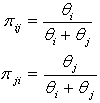 Alternatively the Bradley-Terry Model can be fitted as log linear model (see e.g., 1; 6; 10; 14). Dittrich &Hatzinger[8] fitted the log-linear version of Bradley-Terry[3] Model using R package (see 7) after the formulations of the following equations:
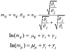 Where the nuisance parameter
  may be interpreted as interaction parameters representing the universities involved in the respective comparisons and the universities related terms are denoted by
2. Modification of Log-Linear Bradley-Terry Model
- The basic Bradley-Terry model is invariant under the change of scale and identification is obtained under the condition:
 Using
Using 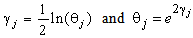 we get,
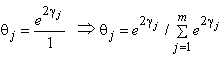 After simplifying; we obtain some modified form, after the log-linear Bradley-Terry model by Dittrich et al.[6], for the estimation of log odds via Bayesian paradigm as below:
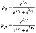 The
The  are the preferences probabilities based on the log odds parameters.
3. Bayesian Inference of the Modified Function
- Bayesian analyses of log-linear models are complicated as we usually perform these analyses using complicated numerical integrations. It is of great practice that the posterior distribution turns out to be an improper density function. Therefore, we consider the non-informative Jeffreys’ prior (see 11 & 4) for the proposed model. This analysis is based on the likelihood function and the prior distribution; we first derive the likelihood and define the prior distribution as below.
3.1. Notations and Likelihood Function
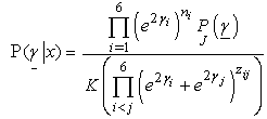
- In the present situation, we see that there are only two possible outcomes of the paired comparison experiment, i.e., either object, ‘Ai’ is preferred to ‘Aj’ or the vice versa. The preference probability
 denotes the probability of object, ‘Ai’ preferred over object ‘Aj’ in all
  fixed number of independent paired comparisons for all of the pair of objects. Random variable
 is assumed to follow a binomial distribution
  and the likelihood function takes the form:
 The
The  is the constraint on the numerical integration and ‘k’ is the normalizing constant and
  is the total number of times object
  is preferred.
3.2. Jeffreys’ Prior Distribution
- The Jeffreys’ prior[11] for the
 is proportional to the square root of determinant of Fisher (9) Information Matrix and given as:
 The
The  The
The  be the ‘p x p’ Fisher[9] information matrix, that is, the logarithm of likelihood functions of parameter space
  and given as follow:
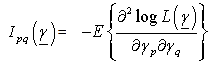 The
The  represents the likelihood function.
3.3. Posterior Distribution for the Model via the Jeffreys Prior
- The joint posterior distribution with the Jeffreys’[11] prior takes the following form
 The
The  is the normalizing constant. The identifiably condition is obtained with:
  We need the following second order partial derivatives of Log-likelihood functions of paired comparison model.
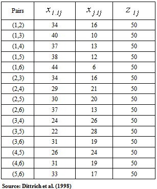
 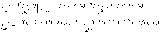 In Table 1, data is taken from Dittrich et al.[6] about students’ preferences for the six European universities as:
|
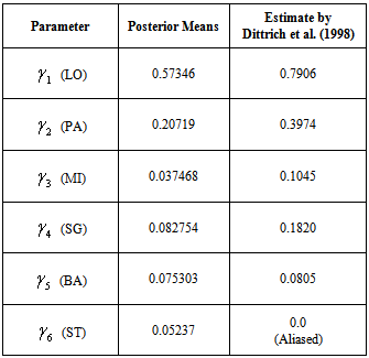
3.4. Bayesian Estimation using Modified Form of the Model Parameters
|
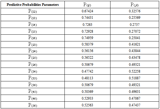
3.5. Posterior Predictive Probabilities Using Jeffrey’s Prior
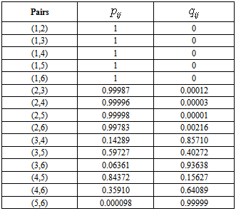
- The predictive probabilities[13] show the preferences for the pair of objects when a single comparison between pair of objects will carry out in the future. The formula for predictive probability for objects Ai and Aj is given as below:
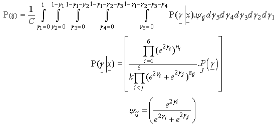 Table 3 shows the posterior predictive probabilities for fifteen pair of objects it also indicates the following relationship between the six universities at the scale of preferences.
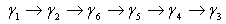
|
3.6. Bayesian Testing of Hypothesis using Jeffrey’s Prior
- The null and alternate hypotheses for pair of objects are
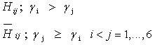 The general formula to calculate the posterior probabilities of null hypothesis for objects Ai with Aj is given below as:
 With
With 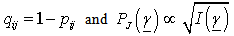 And
And 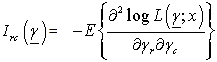 Here
Here 
 And
And 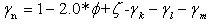 We use the following transformation by Aslam[2] to obtain the posterior probabilities of the hypotheses.
 We follow the decision criteria suggested by Aslam[2]. The criteria are easy to understand that is if any one of the posterior probability of hypothesis either
  or
or  is more than 90%, that hypothesis will be accepted. The posterior probabilities of hypotheses are shown in Table 4. We denote the posterior probabilities by
 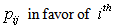 objects and
 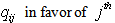 objects. We now interpret each of the tested hypotheses for six parameters. The probability
  shows the strongest favor of London University when compared with Paris University. Also
  has the probability less than 10 %, so we accept the hypothesis
  and conclude that London University has the greater preference probability when compared with Paris University. Now
  has the probability, which is less than 10% so we accept
  and we conclude that London University has the greater preference probability when compared with Milan University. Also the decision for the greater preference probability of London School of Economics and St. Gallen University is inconclusive. Also the decisions for the greater preference probabilities of London School of Economics against Barcelona University and Stockholm School of Economics are inconclusive. The probability for
  is less than 10%, so we accept
  and conclude that Paris University has the greater preference probability when compared with Milan University. The probabilities of
 are less than 10%, so we accept
 concluding that Paris University has the greater preference probabilities when compared with St. Gallen University, Barcelona University and Stockholm School of Economics. The probability for
  is not less than 10%, so we could not accept any of the hypotheses and the decision is inconclusive. The probability for
  is also greater than 10%, so decision is inconclusive. The probability for
  is less than 10 %, so we accept
  and conclude that Stockholm School of Economics has the greater preference probability when compared with Milan University. The probability for
  is not less than 10% so the decision is inconclusive. The probability for
  is not less than 10 %, so the decision is inconclusive. The probability for
  is less than 10 %, so we accept
  and conclude that Stockholm School of Economics has the greater preference probability when compared with Barcelona University.
|
 six null and alternative hypotheses are accepted having the strong probability of acceptance, while as, three hypotheses are remained inconclusive.
3.7. Appropriateness of the Model
- The classical technique of Chi-Square method to test the hypothesis of goodness of fit for the modified form of the model is used. The null and alternate hypotheses are as follow:
 The model is good fit of the data
 The model does not fit the dataWe calculate the expected frequencies by the following formula:
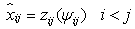 The level of significance is 5% and the test statistic follows the Chi-Square distribution as:
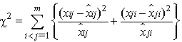 We follow the consideration by Aslam[2) for the choice of degree of freedom by the following formula:
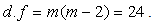 Table 5 shows the observed and expected number of preferences as below in Table 5 as follow:
|

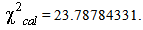 With p-value= 0.473781549.And the table value is:
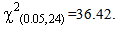 Critical Region is as follow:
 From the critical region, there is no evidence to reject the null hypothesis; therefore, we conclude that the model good fits the data.
4. Conclusions & Discussions
- Bayesian inference using Jeffreys[11] prior produced consistent estimates as compare to the classical approach by overcoming the little deficiency in the estimation of a parameter aliased by the estimation technique of Dittrich et al.[6] (see Table.2). Posterior predictive probabilities for each pair of Universities are obtained in Table. 3. Ranking is ensured in Table.2 through posterior probabilities of hypotheses for each pair of Universities in Table.4.Posterior means for object related parameters
 are obtained for ranking the six European Universities. It could be further generalized for the parameters of ties, order effects, the object specific covariates, subject specific covariates and their interaction parameters via Bayesian inference.