Quang Phung Duy
Department of Mathematics, Foreign Trade University, Ha noi, Viet Nam
Correspondence to: Quang Phung Duy , Department of Mathematics, Foreign Trade University, Ha noi, Viet Nam.
| Email: |  |
Copyright © 2012 Scientific & Academic Publishing. All Rights Reserved.
Abstract
The aim of this paper is to build an exact formula for ruin probability of generalized risk processes under constant interest force with sequences of random variables such that these sequences are usually assumed to be positive integer – valued random variables. An exact formula for finite time ruin (non-ruin) probabilities are derive by using technique of classical probability. A numerical example is given to illustrate results.
Keywords:
Ruin Probability, Non –ruin Probability, Homogeneous Markov Chain
Cite this paper: Quang Phung Duy , Computing Ruin Probability in Generalized Risk Processes under Constant Interest Force, International Journal of Probability and Statistics , Vol. 2 No. 2, 2013, pp. 35-41. doi: 10.5923/j.ijps.20130202.04.
1. Introduction
Claude Lefèvre and Stéphane Loisel[1] studied the problem of ruin in the classical compound binomial and compound Poisson risk models. Their primary purpose is to extend those models which is an exact formula derived by Picard and Lefèvre[9] for the probability of (non-ruin) ruin within finite time. Hong N.T.T. (see [7]) recently built an exact formula for finite time ruin (non-ruin) probability for model:  With
With  are positive integer number.However, Claude Lefèvre and Stéphane Loisel[1] did not provide an exact formula for ruin probability of generalized risk processes under constant interest force with sequences of random variables such that these sequences are usually assumed to be positive integer – valued random variables, with surplus process
  written as
 | (1.1) |
where  is initial surplus (
 ),
), is constant interest (
 ),
), and
and  are positive integer numbers,
  and
and  take values in a finite set of positive integer numbers;
  and
and  are assumed to be independent.With these assumptions, the aim of this paper is to build an exact formula for finite time ruin (non-ruin) probability of model (1.1). In our study, we extended the result of Hong N. T. T for model (1.1) with any r > 0. This is the first time that gives an exact formula for ruin (non-ruin) probability for model (1.1) whose exact formula for finite time ruin (non-ruin) probability are derived by using technique of classical probability.The paper is organized as follows; in Section 2, we build an exact formula for ruin (non-ruin) probability for model (1.1) with
  and
and  being independent and identically distributed positive integer – valued random variables,
  and
and  are assumed to be independent. An extended result in Section 2 with
  and
and  being homogeneous Markov chains is given in Section 3. A numerical example is give to illustrate these results in Section 4. Finally, we conclude our paper in Section 5.
2. Computing Ruin Probability of Generalized Risk Processes under Constant Interest Force with Sequences of Independent and Identically Distributed Random Variables
Let model (1.1). We assume that:Assumption 2.1. u and t are positive integer numbers.Assumption 2.2  is a sequence of independent and identically distributed random variables,
  take values in a finite set of positive integer numbers
 with
with  ,
, .Assumption 2.3
  is a sequence of independent and identically distributed random variables,
  take values in a finite set of positive integer numbers
  with
with  ,
, .Assumption 2.4
  and
and  are assumed to be independent.From (1.1), we have:
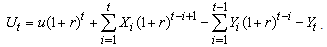 | (2.1) |
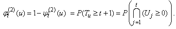
Supposing that the ruin time is defined by , where
  .We define the finite time ruin (non-ruin) probabilities of model (1.1) with Assumption 2.1 to Assumption 2.4, respectively, by
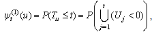 | (2.2) |
 | (2.3) |
Throughout this paper, we denote  if
if  To establish a formula for
  , we first proof the following Lemma.Lemma 2.1. Any u and
  are positive integer numbers.With
  being a positive integer number and
  satisfies:
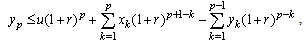 | (2.4) |
then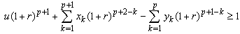 | (2.5) |
Proof.From (2.4), we have Implies
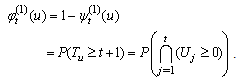
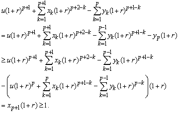 Hence (2.5) holds.This completes the proof.Next, we give an exact formula for finite time non-ruin (ruin) probability of model (1.1).Theorem 2.1. Let model (1.1) satisfy Assumption 2.1 to Assumption 2.4, then finite time non-ruin probability of model (1.1) is defined by
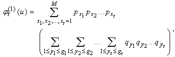 | (2.6) |
where ,
, ,…
,… ,In addition,
  is integer part of the
  .Proof.Firstly, we have


 | (2.7) |
By Assumption 2.2, we let  with
with  being positive integer numbers and satisfying:
  . Let
. Let .Since
  is a sequence of independent random variables then
 | (2.8) |
Hence, (2.7) is given | (2.9) |
where | (2.10) |
By Assumption 2.3, we let  with
with  being positive integer numbers andsatisfying:
  . Let
. Let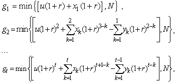 In addition,
  is integer part of
  ,By using Lemma 2.1,
  ,
,  , …,
, …,  are integer numbers.Thus, (2.10) is written as
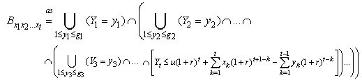 | (2.11) |
As Assumption 2.3, we let  with
with  is positive integer number then
  . Combining Assumption 2.3, (2.10) and formulas define
  , we have
 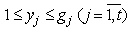 .Therefore, (2.11) can be rearranged as
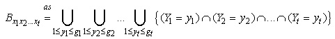 | (2.12) |
For the reason that  is a sequence of independent random variables then
 In the other hand, system of events
 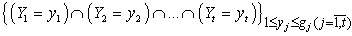 in (2.12) is incompatible then
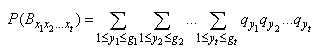 | (2.13) |
Next, we consider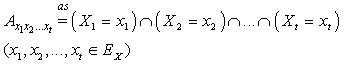 and
and By using,
  and
and  are independent, if
  and
and  hold then
  and
and  are independent events. In addition, system of events
 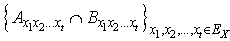 in (2.9) is incompatible. Therefore, combining (2.8) and (2.13), we have
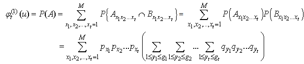 | (2.14) |
This completes the proof.Corollary 2.1. Let model (1.1) satisfy Assumption 2.1 to Assumption 2.4, then finite time ruin probability of model (1.1) is defined by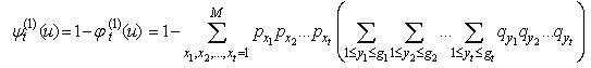 | (2.15) |
Remark 2.1. Formula (2.6) (or (2.15)) gives a method to compute exactly finite time non-ruin (ruin) probability of model (1.1) which  and
and  are sequences of independent and identically distributed random variables, and they take values in a finite set of positive integer numbers.
3. Computing Ruin Probability of Generalized Risk Processes under Constant Interest Force with Homogeneous Markov Chains
Let model (1.1). We assume that:Assumption 3.1.  are positive integer numbers.Assumption 3.2.
  is a homogeneous Markov chain,
  take values in a finite set of positive integer numbers
  with
with  where
where  . In addition,
 .Assumption 3.3.
  is a homogeneous Markov chain,
  take values in a finite set of positive integer numbers
  with
with  where
where  . In addition,
  Assumption 3.4.
  and
and  are assumed to be independent.Supposing that the ruin time is defined by
 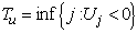 where
where  .We define the finite time ruin (non-ruin) probability of model (1.1) using Assumption 3.1 to Assumption 3.4, respectively, by
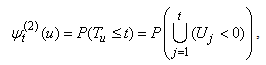 | (3.1) |
 | (3.2) |
Similar to Theorem 2.1, we haveTheorem 3.1. Let model (1.1) satisfy Assumption 3.1 to Assumption 3.4, then finite time non-ruin probability of model (1.1) is defined by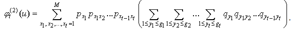 | (3.3) |
where,  is defined in the same way with Theorem 2.1.Proof.We proof similarly as Theorem 2.1, where, (2.8) replaced by
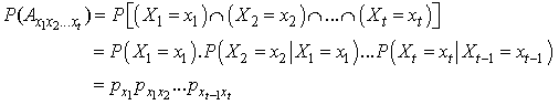 In the other hand, we have
 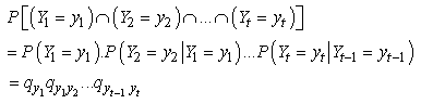 In addition, (2.13) substituted by
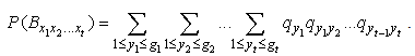 By using the same method to prove Theorem 2.1, we have formula (3.3).This completes the proof.Corollary 3.1. Let model (1.1) satisfy Assumption 3.1 to Assumption 3.4, then finite time ruin probability of model (1.1) is defined by
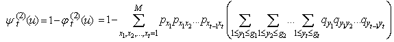 | (3.4) |
Remark 3.1. Formula (3.3) (or (3.4)) gives a method to compute exactly finite time non-ruin (ruin) probability of model (1.1) which  and
and  are homogeneous Markov chains and they take values in a finite set of positive integer numbers.
4. Numerical Illustration
4.1. Numerical Illustration for 
Let  be a sequence of independent and identically distributed random variables,
  take values in a finite set of positive integer numbers
 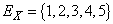 with
with  having a distribution:
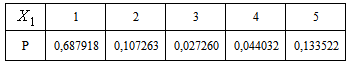 Let
Let  be a sequence of independent and identically distributed random variables,
  take values in a finite set of positive integer numbers
  with
with  having a distribution:
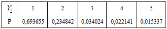 By using the C progaram, the
  is calculated with the assumptions above of random variables
  .Table 4.1 shows
  for a range of value of u.
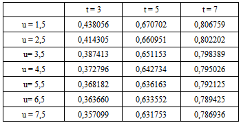
Table 4.1. Ruin probabilities of model (1.1) with Assumption 2.1- 2.4 and r = 0,15
 |
| |
|
4.2. Numerical Illustration for 
Let be a homogeneous Markov chain,
  take values in a finite set of positive integer numbers
 ,with
,with  having a distribution
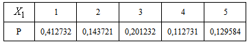 In addition, matrix
  is given by
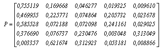 Let
Let  be a homogeneous Markov chain,
  take values in a finite set of positive integer numbers
 , with
  having a distribution
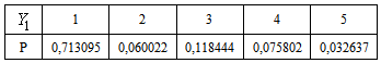 In addition, matrix
  is given by
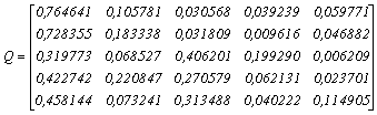 By using the C progaram, the
  is calculated with the assumptions above of random variables
  and matrixs
  .Table 4.2 shows
  for a range of value of u.
Table 4.2. Ruin probabilities of model (1.1) with Assumption 3.1-3.4 and r = 0,15
 |
| |
|
5. Conclusions
By using technique of classical probability with  , claims, premiums all are positive integer numbers and
  is a positive number, this paper constructed an exact formula for ruin (non-ruin) probability of model (1.1), where sequences of claims and premiums are independent and identically distributed random variables or homogeneous Markov chains. Our main results in this paper not only prove Theorem 2.1 and Theorem 3.1 but also give numerical examples to illustrate for Theorem 2.1 and Theorem 3.1. These results proof for the suitability of theoretical results and practical examples. It also mean that:When initial
  is increasing then
  ,
, are decreasing,With
  being unchanged, when
  is increasing then
  ,
, are increasing.
ACKNOWLEDGMENTS
The authors are thankful to the referee for providing valuable suggestions to improve the quality of the pape.In addition, the author would like to thank my advisor, Professor Bui Khoi Dam for his patient guidance, encouragement and advice.
References
| [1] | Claude Lefèvre, Stéphane Loisel, On finité - time ruina probabilities for classical models, Scandinavian Actuarial Journal, Volume 2008, Issue 1, (2008), 56-68. |
| [2] | De Vylder, F. E., La formule de Picard et Lefèvre pour la probabilité de ruine en temps fini, Bulletin Francais d’Actuariat, 1, (1997), 31-40. |
| [3] | De Vylder, F. E., Numerical finite – time ruin probabilities by the Picard – Lefèvre formula. Scandinavian Actual Journal, 2, (1999), 97-105. |
| [4] | De Vylder, F. E. and Goovaerts, M. J., Recursive calculation of finite – time ruin probabilities, Insurance: Mathematics and Economics, 7, (1998), 1-7. |
| [5] | De Vylder, F. E. an d Goovaerts, M.J., Explicit finite – time and infinite – time ruin probabilities in the continuous case. Insurance: Mathematics and Economics,24, (1999)155-172. |
| [6] | Gerber, H.U., An Introduction to Mathematical Risk Theory. S. S. Huebner Foundation Monograph, University of Philadelphia: Philadelphia. Insurance: Mathematics and Economics, 24, (1979),155-172. |
| [7] | Hong, N.T.T, On finite – time ruin probabilities for general risk models. East-West Journal of Mathematics: Vol.15, No1 (2013), pp.86-101. |
| [8] | Ignatov, Z.G., Kaishev, V. K. and Krachunov, R. S., An improved finite – time ruin probability formula and its Mathematica implementation. Insurance: Mathematics and Economics, 29, (2001), 375-386. |
| [9] | Ignatov, Z.G., Kaishev, V. K., A finite – time ruin probability formula for continuous claim severities. Journal of Applied Probability, 41,(2004), 570-578. |
| [10] | Picard, Ph. and Lefèvre, Cl., The probability of ruin in finite time with discrete claim size distribution. Scandinavian Actuarial, (1997), 58 – 69. |
| [11] | Rullière, D. and Loisel, St., Another look at the Picard – Lefèvre formula for finite – time ruin probabilities. Insurance: Mathematics and Economics,35,(2004),187-203. |
 Abstract
 Reference
 Full-Text PDF
 Full-text HTML