1. Introduction

A wide number of research studies have being carried out to study the trends and growth rates of agricultural production of different crops based on linear, non-linear, time series and nonparametric regression models viz. (Panse[24], Dey[4], Reddy[25], Narian et al.,[19], Kumar and Rosegrant[14], Kumar[15], Joshi and Saxena[11], Singh and Srivastava[28], Shah et al.,[29], Patil et al.,[22]).

In practice, a suitable parametric models such as linear, non-linear and time series models may not be available to estimate the locations of jump points and corresponding sizes of jump values of the selected regression models.Whenever there is no appropriate parametric method available, we may start from nonparametric regression.

In applications of regression methods, we are often interested in the locations of jump points and thecorresponding sizes of jump values of the regression function. For example, when studying the impact of advertising, the time at which this action takes effect could effectively be modeled by the location of a jump point and the magnitude of the effect of this action is measured by the size of the jump. If we ignore the existence of the jump point, then we may make a serious error in drawing inferences about the process under study (Wu and Chu[31]).

The parametric (non-linear regression) and nonparametric regression techniques represent two different approaches to the problem of regression analysis. This does not mean that the use of one precludes the use of the other. Parametric regression requires very specific, quantitative information about the functional form. Such techniques are mostappropriate when theory, past experiences or other sources are available to provide detailed knowledge about the process under study. In contrast, nonparametric regressiontechniques require only qualitative information about the functional form and actual let data speak for it concerning the actual form of the regression function. The best suited methods are the ones where there is little or no prior information available about the regression function (Hardle[7]).

In recent years, nonparametric regression technique for functional estimation has become increasingly popular tool for data analysis. The technique imposes only fewassumptions about shape of function and therefore, it may be more flexible than usual parametric approaches. In many situations, one may not know the exact functional form and sometimes there may not be any parametric functional form to represent the data. In such situations, the nonparametric technique, which entirely depends on the data, will be more suitable. This method is based on the local regression smoother and only assumption about the form of trend. The increased data availability and explosion of computing power have now made it possible to use a wide range of modern nonparametric regression techniques in time-series data.

By considering the above facts in mind, the present investigation is planned to use both parametric andnonparametric regression models to study the trends and growth rate in area, production and productivity of tobacco crop grown in Middle Gujarat region, India with the following objectives.

i. To study the trends in area, production and productivity based on different non-linear and nonparametric regression models and

ii. To examine jump points and its sizes in area, production and productivity using nonparametric regression techniques.

2. Materials and Methods

To achieve the stipulated objectives, the present study had been carried out on the basis of time-series data on area, production and productivity of tobacco crop pertaining to the period 1949-50 to 2008-09 had been collected through the Gujarat government official web site www. agri. gujarat. gov.in.

2.1. Non-linear Regression Models

Statistical modelling essentially consists in constructing a model, represented by a set of equations to describe the input-output relationship among the variables of interest. From a realistic point of view, such relationship among variables in agriculture and biological sciences is ‘non-linear’ in nature. In such a model, a unit increase in the value of independent variable(s) may not result in an equivalent unit increase in the dependent variable. A non-linear regression model is one in which at least one of the parameters appears non-linearly. A non-linear model, which can be transformed into linear model by some transformation is called “intrinsically linear”, else it is called as “intrinsically non-linear”. Mathematically, in non-linear models at least one of the derivatives of the expectation function with respect to at least one parameter is a function of parameter(s). The model

is a non-linear regression model as the derivatives of Y_x with respect a and b are both functions of a and /or b. Details about the family of non-linear models are mentioned in Bard[2], Seber and Wild[26], Ratkowsky[24], Draper and Smith[5] and Montgomery et al.,[17]. Like in linear regression, parameters in a non-linear model can also be estimated by the method of least squares. However, due to the difficulty in the procedure of computation, the common practice is to work with the log transformed model.

The log transformation is valid only when error term ‘e’ in the above equation is multiplicative in nature. Thereafter, method of least square is used to estimate the unknown parameters. Furthermore, R² value is calculated to measure the goodness of fit of the model.

The log transformed procedure suffers from some important drawbacks.

a). Original structure of the error term got disturbed due to transformation.

b). R² values computed, assess the goodness of fit of the transformed model and not of the original non-linear model.

c). Proceeding further to carryout residual analysis for the residuals generated by the transformed model, will result in erroneous conclusion.

As a remedy to these pitfalls, non-linear regression procedures are already developed in literature which necessitates computer intensive tools to find solution for the parameters (Venugopalan and Shamasundaran[30]). The following non-linear models are considered in the present investigation.

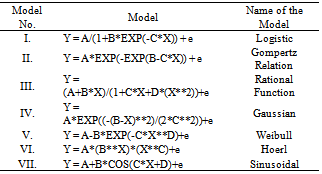where Y is the area/production/productivity during the time X; A, B ,C and D are the parameters, and e is the error term. The parameter ‘C’ is the intrinsic growth rate and the parameter ‘A’ represents the carrying capacity for each model. Symbol B represents different functions of the initial value Y(0) and d is the added parameter. In addition to the above non-linear models some other non-linear models also are employed as per the data need.

Four main methods are available in literature (Seber and Wild[26]) to obtain estimates of the unknown parameters of a non-linear regression model. These are: (i) Gauss-Newton method (ii) Steepest-Descent method (iii)Levenberg-Marquardt technique and (iv) Do not use derivative (DUD) method. However, in all these methods the following steps are carried out.

Step (i). Starting with a good initial guess of the unknown parameters, a sequence of θ’s which hopefully converge to θ is computed.

Step (ii). Error sum of squares or objective function expressed as is minimized with respect to the current value of θ. The new estimates are obtained.

Step (iii). By feeding the recently obtained estimates as the initial guess for the next iteration, objective function S(θ) is minimized again to obtain fresh estimates. This procedure is continued till the successive iteration yielded parameter estimate values are close to each other.

2.1.1. Choice of Starting Values of the Parameters for Various Models

All the iterative procedures require initial values θ_r0 (r = 1, 2, 3,…, p) of the parameter θ_r. The choice of good initial values can spell the difference between success and failure in locating the fitted value or between rapid and slow convergence to the solution. Also, if multiple minima exist in addition to absolute minimum, poor starting values may result in convergence to an unwanted stationary point of the sum of squares surface (Bard[2]). This unwanted point may have parameter values which are physically impossible or which does not provide the true minimum value of S(θ).There are number of ways to determine initial parameter values for non-linear models. The most obvious method for making the initial guesses is by the use of prior information. Estimates calculated from previous experiments, known values from similar systems, values computed fromtheoretical considerations: all these form ideal initial guesses. In this study the Curve expert Ver.1.3 software package is used to estimate the initial values.

2.1.2. Measures of Goodness of Fit

To test the goodness of fit of the fitted polynomial model, the co-efficient of determination R² defined as the proportion of total variation in the response variable (time) being explained by the fitted model is widely used.

R² = .

To test the overall significance of the model the F test is used.

F=

which follows F distribution with k (number of parameter in the model), (n-k-1) degrees of freedom. The individual regression co-efficient is tested using the t test t= which follows t – distribution with (n-k-1) degrees of freedom, b_j = estimated j^th co-efficient and s.e.(b_j) is the standard error of b_j .

In addition to the above, two more reliability statistics viz., Root Mean Square Error (RMSE) and Mean Absolute Error (MAE) are generally utilized to measure the adequacy of the fitted model and it can be computed as follows:

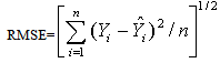and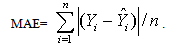

The lower the values of these statistics, the better is the fitted model.

Before taking any final decision about the appropriateness of the fitted model, it is of paramount importance to investigate the basic assumptions regarding the error term, viz., randomness and normality. Normality of residuals is examined by using Shaprio-Wilks test (Agostid’no and Stephens[1]). Further, to test the presence or absence of autocorrelation in the data set Durbin-Watson test procedure (Lewis-Beck[13]) is utilized.

2.2. Nonparametric Regression Model (Hardle[7]; Jose et al.,[10])

The nonparametric regression model with the additive error of the form

(2.2.1)

where y_i is the observation (area, production and productivity) of the i^th time point, m is the trend function, which is assumed to be smooth, and are random errors with mean zero and finite variance . The kernel weighted linear regression smoother (Fan[6]) is used to estimate the trend function non parametrically. The value of the local linear regression smoother at time x is the solution of a₀ to the following weighted least squares problem:

where K is a bounded symmetric kernel density function and h is the bandwidth. Let and be the solutions to the weighted least squares problem. The estimate of the trend function m(t) is given by

where

and

The optimum bandwidth h can be obtained by the method of cross-validation. The slope m^|(x) of m(x) can be considered as the simple linear growth rate at the time point x. The estimate of m^|(x) is given by

Where

Under the assumption that the trend function m is smooth and m(x) ≠ 0 for all x [0,1], the value of the relative growth rate at time X can be written as :

Since and , a consistent estimate of the relative growth rate r_x is given by :

Taking arithmetic mean, the requisite compound growth rate over a given time-period may be obtained.

2.3. Estimation of Change Points

To estimate the trends and growth rate the function should be smooth. But in many situations there exist sudden changes or jumps in the trend and/or growth rates. Local linear regression smoother is used to obtain a smooth fit of a regression or trend function. The estimators of the location and size of change points in a function are obtained by fitting local linear regression with dummy variables for the jumps. This method does not require that the number and order of jumps to be known in advance as do most other existing methods Loader[16] and Muller[18]. Other related works can be found in Jose and Ismail ([8],[9]) and Bowman et al.,[3].

A jump point for the regression model (, i=1,…,n) at τ [h, 1-h] with jump sizes and for the function m and its slop m’, respectively, is defined in the following sense m (τ +) – m (τ) = and m’ (τ +) – m’ (τ) =

For any change point τ, we have some i, 1 ≤ i ≤ n, such that t_i ≤ τ ≤ t_i+1. However, the data cannot be used to distinguish possible changes in the interval. Therefore we assume that the change points occur at any of the design points in the interval[h, 1−h] and the distance between any two change points is greater than h.

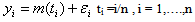(2.3.1)

Let there exist a jump point in the above regression model at t_τ [h, 1-h] with jump sizes and for the function m and its slop m^|, respectively, then the minimization problem

becomes Minimize

where I is the indicator function and be the coefficient vector.

To estimate the change point, fit the following weighted least squares regression corresponding to all t_k [h, (1−h)]:

Minimize

The solution to the above weighted least squares problem is given by:

where,

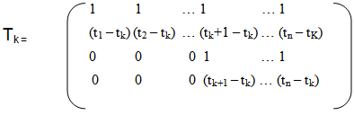
and Y’ =[y₁ y₂ … y_n]

The regression sum of squares due to is given by:

The residual sum of squares is given by:

The ratio of the mean regression sum of squares of to the mean residual sum of squares with t = t_k is given by :

The estimate of the jump points is given by:

and the corresponding estimates of the coefficient vector be the estimates of the jump sizes. The above procedure can easily be extended to the case of more than one jump point. Let there be q jump points for the regression function m and/or its derivative at t_τj, j=1… q, then the estimates of the change points are given by:

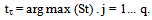
where

and the corresponding estimates of the co-efficient vector ∆ =[ ] be the estimates of the jump sizes. If the number of jump points is not known in advance the above sequential procedure continues for j=1,..., p(say), where p is fixed in such a way that the max(s_t), t∈ A_P is greater than or equal to its critical value C_x(p) and max(s_t) . Here, t∈ A_{P +1} is less than its critical value C_x(p + 1).

3. Discussion

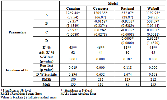
Different non-linear and nonparametric regression models were employed to study the trends in area, production and productivity data of tobacco crop. The characteristics of fitted non-linear models are presented (Table 2, Table 3 and Table 4). The findings are discussed in sequence as under.

3.1. Trends in Area Based on Non-linear Models

The result presented in Table 2 for the area under the cultivation of tobacco crop revealed that among the different non-linear models fitted, the maximum adjusted R² of 80% was observed in case of Rational function with the minimum values of RMSE (129) and MAE (95) in comparison to that of other non-linear models. The Shapiro-Wilks test (test for normality) statistic of 0.972 (df = 60) which gives p=0.182 and the Run test (test for randomness) value of 4.10 which gives p=0.118 indicating that the residuals were normally and independently. All the estimated values of the parameters in this model were found to be within the 95% confidence interval indicating that the parameters were significant at 5% level of significance. Among the non-linear models fitted to the area under the tobacco crop, the following rational function was found suitable to fit the trends.

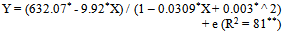(3.1.1)

Table 2. Characteristics of fitted Non-Linear models for area under the tobacco crop

Table 3. Characteristics of fitted Non-Linear models for production for production of tobacco crop

Table 4. Characteristics of fitted Non-Linear models for yield of the tobacco crop

3.2. Trends in Production Based on Non-linear Models

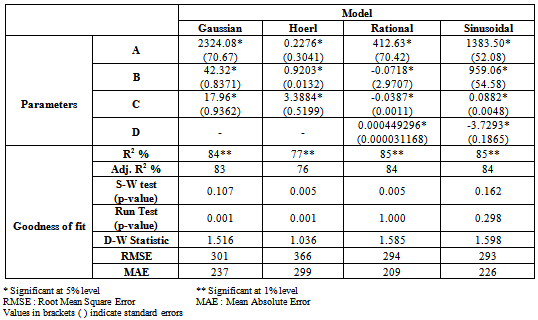
For the production of tobacco crop, the Sinusoidal model had highest R2 (84%) with the comparatively lower values of RMSE (293) and MAE (226). Also the residuals were found to be independently normally distributed because the p-values of run test and Shapiro-Wilks were non-significant. All the estimated values of the parameters in these models were found to be within the 95% confidence interval indicating that the parameters were significant at 5% level of significance. Among the non-linear models fitted the following Sinusoidal model was found suitable to fit the trends in production of the tobacco crop.

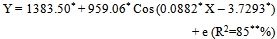(3.2.1)

3.3. Trends in Productivity Based on Non-linear Models

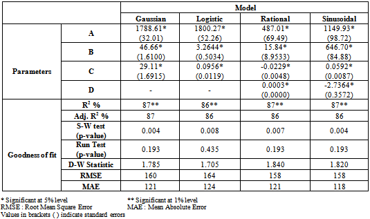
In case of productivity of tobacco crop, again the Sinusoidal models had highest adjusted R² of 86 per cent with comparatively lower values of root mean square (158) and mean absolute errors (118) in comparison to that of other non-linear models. All the parameters were found to be significant. However the Shapiro-Wilks test value 0.937 with p-value 0.004 was found to be significant the residuals due to this model were not normally distributed and hence none of the non-linear models were found suitable to fit the trends in productivity of tobacco crop.

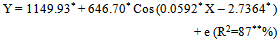(3.3.1)

Patel et al.,[21], Kalola et al.,[12] and Sarma[27] used first degree polynomial model to study the trends in tobacco crop grown in different states in India. In all these studies the test for normality and randomness of the residuals were not reported. The tests for normality as well as randomness are essential for the model to be an appropriate for the study.

3.4. Trends in Area, Production and Productivity Based on Nonparametric Regression Model

Using the cross-validation method, for the area,production and productivity of the tobacco crop, the optimum bandwidth have been computed as 0.08, 0.1 and 0.12, respectively. Nonparametric estimates of underlying growth function were computed at each and every time points. Residual analysis showed that the assumptions ofindependence or errors were not violated at 5% level of significance. The RMSE and MAE values were for area 32.28 and 24.27; for production 59.34 and 47.87; productivity 27.76 and 19.71, respectively. These values were much lower than those obtained through the non-linear models, indicating thereby the superiority of this approach over the parametric approach. The nonparametric regression model was selected as the best fitted trend function for the area, production and productivity of tobacco crop.

The trend function for the area indicates that there was an increasing trend up to 1958-59. Also it was found that there was a sudden shift in the trend and growth rate during the year 1959-60 (Figure 1). The area had been increased by an amount of 19300 hectares.

Similarly the production trend function of tobacco crop indicates increasing trend (Figure 2) up to 1973-74 and then there was a sudden increasing shift in production by an amount 24900 metric ton have been observed.

In case of productivity there has been an increasing trend up to 1980-81 and then sudden increase in productivity by an amount of 305 kg/ha was observed (Figure 3). This might be due to a technology mission introduced by the government. These kind of changes can not be observed in the case of growth rate estimated using the traditional parametric approach.

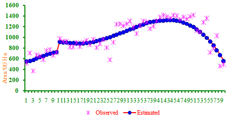Figure 1. Trends in Area based on nonparametric regression

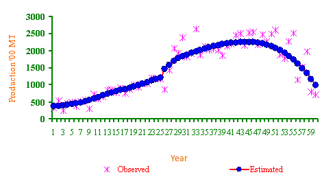Figure 2. Trends in Production based on nonparametric regression

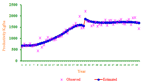Figure 3. Trends in Productivity based on nonparametric regression

4. Conclusions

None of the non-linear models were found suitable to fit the trends in area, production and productivity where there exists a jump points in the data set. The nonparametric regression have emerged as the best fitted trend function to locate the jumps and amount of jumps presents in the area, production and productivity of the data set.

ACKNOWLEDGMENTS

The authors are thankful to the referee for providing valuable suggestions to improve the quality of the paper. The financial assistance received by the second author in the form of Junior Research Fellowship from University Grant Commission (UGC), India is highly acknowledged.