-
Paper Information
- Next Paper
- Paper Submission
-
Journal Information
- About This Journal
- Editorial Board
- Current Issue
- Archive
- Author Guidelines
- Contact Us
International Journal of Probability and Statistics
p-ISSN: 2168-4871 e-ISSN: 2168-4863
2013; 2(1): 1-8
doi:10.5923/j.ijps.20130201.01
Estimation of Partially Accelerated Life Tests for the Extreme Value Type-III Distribution with Type-I Censoring
 Abstract
 Reference
 Full-Text PDF
 Full-text HTML
S. Saxena, S. Zarrin
Department of Statistics & Operation Research Aligarh Muslim University, Aligarh, India
Correspondence to: S. Saxena, Department of Statistics & Operation Research Aligarh Muslim University, Aligarh, India.
| Email: |  |
Copyright © 2012 Scientific & Academic Publishing. All Rights Reserved.
In this paper a constant stress Partially Accelerated Life Test (CSPALT) using type-I censoring is obtained for Extreme Value Type-III distribution. This distribution has been found appropriate for high reliability components. Maximum Likelihood (ML) Estimation is used to estimate the parameters of CSPALT model. Confidence intervals for the model parameters are constructed. CSPALT plan is used to minimize the Generalized Asymptotic Variance (GAV) of the ML estimators of the model parameters.
Keywords: Acceleration Factor, Constant Stress, Fisher Information Matrix, Generalized Asymptotic Variance, Optimum Test Plan, Maximum Likelihood Estimation, Confidence Intervals
Cite this paper: S. Saxena, S. Zarrin, Estimation of Partially Accelerated Life Tests for the Extreme Value Type-III Distribution with Type-I Censoring, International Journal of Probability and Statistics, Vol. 2 No. 1, 2013, pp. 1-8. doi: 10.5923/j.ijps.20130201.01.
Article Outline
1. Introduction
- In traditional life testing and reliability experiments, researchers used to analyse time-to-failure data obtained under normal operating conditions in order to quantify the product’s failure-time distribution and its associated parameters. However, such life data has become very difficult to obtain as a result of the great reliability of today’s products, and the small time period between design and release. This problem has motivated researchers to develop new life testing methods and obtain timely information on the reliability of product components and materials. ALT is then adopted and widely used in manufacturing industries. In such testing situations, products are tested at higher-than-usual levels of stress (e.g., temperature, voltage, humidity, vibration or pressure) to induce early failure. The life data collected from such accelerated tests is then analysed and extrapolated to estimate the life characteristics under normal operating conditions. It is useful to divide accelerated tests into two aims (i) During product development, a small number of prototype specimens are forced to fail at high stress. Engineers examine the specimens to identify the causes of failure, and then determine how to improve the product to eliminate or reduce those causes. For thousands of years, engineers have improved product reliability with such development testing, called ESS and HALT. Such testing depends on qualitative engineering knowledge of the product and usually does not involve a physical-statistical model. (ii) After product development, a statistical sample of specimens is tested at high stress levels to measure reliability, that is, to estimate the product life distribution or degradation at lower design stress levels. Such estimation requires a suitable model.In some cases, such life stress relationships are not known and cannot be assumed, i.e., the data obtained from ALT cannot be extrapolated to use condition. So, in such cases, another approach can be used, which Is PALT. In PALT, test units are run at both usual and higher-than usual stress conditions. PALT results in shorter lives than would be observed under normal operating conditions. According to Nelson[1] stress can be applied in a number of ways, commonly used methods are step stress and constant stress. In first case, to use PALT, a test item is run at use condition and, if it does not fail for a specified time, then it is run at accelerated condition until failure occurs or the observation is censored while in second case, PALT can be applied by running each item at either normal use or accelerated condition only, i.e. each unit is run at a constant stress level until the test is terminated. The object of a PALT is to collect more failure data in a limited time without using high stresses necessarily to all test units. Many authors have studied PALT. For an overview of PALT with Type-I censoring, Bai and Chung[2] discussed both, the problem of estimation and optimally designing PALT for test items having an exponential distribution. For items having log-normally distributed lives, PALT plans were developed by Bai, Chung and Chun[3]. Ghaly et al.[4] discussed the problem of parameter estimation for Pareto distribution using PALT in case of type-I censoring. Concerning the constant stress PALT, there are some studies on the optimally designing constant stress PALT, see Bai and Chung[2], Bai, Chung and Chun[3] and Ismail[5]. Attia[6] considered the estimation problem of the Weibull distribution parameters using the ML method. Abdel-Ghani [7] considered only the estimation problem in constant stress PALT for Weibull distribution. Extreme Value distribution arise as limiting distributions for maxima and minima (extreme values) of a sample of independent and identically distributed random variables, as the sample size increases. EVT is the theory of modelling and measuring events which occur with very small probability. This implies its usefulness in risk modelling as risky events per definition happen with low probability. Thus, these distributions were important in Statistics. These models, along with the generalized Extreme Value distribution are widely used in risk management, finance insurance, economics, hydrology, material sciences, telecommunications, and many other industries are dealing with extreme events.In this paper, the problems of both, estimation and optimal design constant stress PALT are considered under Extreme Value type-III distribution using type-I censoring. The constant stress testing has several advantages, see Nelson[1]. ALT model for constant stress are better developed for some material and products. Also it is easier to maintain a constant stress level and data analysis for reliability estimation is well developed.
2. The Extreme Value Distribution: As a Lifetime model
- The Extreme Value type-III distribution has been successfully employed for frequency analysis of low river flows, see Gumble[8].If a random variable
 is said to have an Extreme Value type-III distribution then its probability density function is given by
 | (2.1) |
 | (2.2) |
 | (2.3) |
2.1. CSPALT: Test Procedure
- In a constant-stress PALT, all of the
 items are divided into two parts.
  items are randomly chosen among
  items, which are allocated to accelerated conditions and the remaining
  are allocated to normal use conditions, then each test item is run until
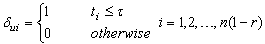
  and the test condition is not changed.Some assumptions are also made in a constant-stress PALT.• The lifetimes
  and
and , of items allocated to normal and accelerated conditions, respectively, are i.i.d. random variables.• The lifetimes
  and
and  are mutually statistically independent.
3. Parameter Estimation: MLE Technique
- The MLE is one of the most important and widely used methods in statistics. It is commonly used for the most theoretical model and kinds of censored data see Grimshaw[9]. The idea behind the maximum likelihood parameter estimation is to determine the estimates of the parameter that maximizes the likelihood of the sample data. Also the MLEs have the desirable properties of being consistent and asymptotically normal for large samples. Also, Bugaighis[10] showed that the ML procedure generally yields efficient estimatorsIn a simple CSPALT, the test item is run either at use condition or at accelerated condition only. A simple constant stress test uses only two stresses and allocates the n sample unit to them; see Miller and Nelson[11].Since the lifetimes of test items follow the Extreme Value distribution of type-III, the probability density function of an item tested at use condition is given by:
 | (3.1) |
 | (3.2) |
 The likelihood function for
 is given by
 | (3.3) |
 is given by
 and the total likelihood function for
  is as follows
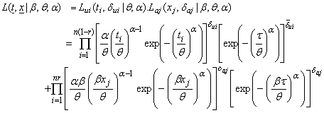 | (3.4) |
 and,
and, 
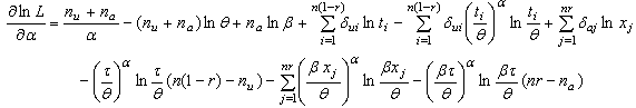
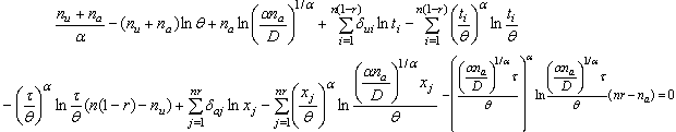
 As it is easier to maximize the natural logarithm of the likelihood function rather than the likelihood function itself. The first derivatives of the natural logarithm of the total likelihood function in (3.4) with respect to
 ,
, and
and  are given by
 | (3.5) |
 | (3.6) |
 | (3.7) |
 ,
, and
and  which solve the equations obtained by letting each of them be zero. So, from (3.5), the ML estimate of
 is given by
 | (3.8) |
 By substituting for
  into (3.6) and (3.7) and equating each of them to zero, the system equations are reduced into the following non linear equations
  | (3.9) |
 | (3.10) |
 and
and . Thus, once the values of
  and
and .are determined, an estimate of
  can be obtained from eq. (3.8). But the exact mathematical expression for the expectation is too difficult to find. So it can be approximated by numerically inverting the asymptotic fisher information matrix. It is composed of the negative second and mixed derivatives of the normal logarithm of the likelihood function evaluated at the MLE. So, asymptotic fisher information matrix can be written as follows
 The elements of Fisher information matrix can be expressed by the following equations


4. Confidence Intervals for the Model Parameters
- The most common method to set confidence bounds for the parameters is to use asymptotic normal distribution of maximum likelihood estimators, see Vander Wiel and Meeker[12].To construct a confidence interval for a population parameter
 ; assume that
 and
and  are functions of the sample data
  such that
  | (4.1) |
 is called a two sided
  confidence interval for
 .
. and
and are the lower and upper confidence limits for , respectively. The random limits
  and
and  enclose
  with probability
 .Asymptotically, the maximum likelihood estimators, under appropriate regularity conditions are consistent and normally distributed. Therefore, the two sided approximate
  confidence limits for a population parameter can be constructed such that:
 | (4.2) |
 is the
  standard normal percentile. Therefore, the two sided approximate
  confidence limits for
 ,
, and
and  are given respectively as follows:
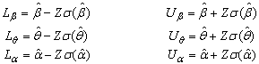
5. Optimum Simple Constant Stress Plan
- In most of the test plans, the same number of test units is allocated to each stress. Such test plans are usually inefficient for estimating the mean life of design stress, see Yang[13]. In this section, statistically optimum test plans are developed to decide optimum sample proportion allocated to each stress. Therefore, to determine the optimum sample proportion
 allocated to accelerated condition,
  is chosen such that the GAV of the ML estimators of the model parameters is minimized. The GAV of the ML estimators of the model parameters as an optimality criterion is commonly used and defined below as the reciprocal of the determinant of the Fisher information matrix
  (Bai, Kim and Chun,[14]).
 The Newton-Raphson method can be applied to numerically determine the best choice of sample proportion allocated to accelerated condition which minimizes the GAV as defined before. Accordingly, the corresponding expected optimum number of items failed at use and accelerated conditions can be obtained, respectively, as follows:
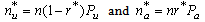 Where
Where And
And
6. Simulation Studies
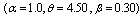
- The data in Table 1 and Table 2 gives the MSE, RABs, RE and variance of the estimators for two sets of parameters
 and
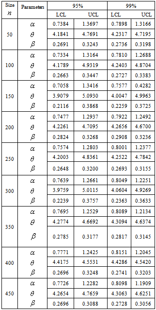
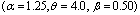
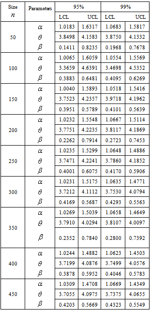
and  respectively. While Table 3 and Table 4 presents the approximated two sided confidence limits at
  and
and  level of significance for the scale parameter and the acceleration factor.From these tables it is concluded that for the first set of parameters
 , the ML estimates have good statistical properties than the second set off parameters
  for all sample sizes. Also as the acceleration factor increases the estimates have smaller MSE and RE. As the sample size increases the RABs and MSEs of the estimates of parameters decrease. This indicates that the ML estimates provide asymptotically normally distributed and consistent estimators for the scale parameter and the acceleration factor.When the sample size increases, the interval of the estimators decreases. Also the intervals of the estimators at
  is smaller than the interval of estimators at
 . Tables are given in appendix.
Notations
 : Total number of test items in a PALT
 : censoring time of a PALT
 : Lifetime of an item at use condition
 : Lifetime of an item at accelerated condition
 : Acceleration factor
 : Probability that an item tested only at use condition fails by
 : Probability that an item tested only at accelerated condition fails by
 : implies a maximum likelihood estimate
 : scale parameter of Extreme Value distribution
 : shape parameter of Extreme Value distribution
 : observed life time of item
  tested at use condition
 : observed life time of item
  tested at accelerated condition
 : Indicator function at use condition
  : Indicator function at accelerated condition
  : Proportion of sample units allocated to accelerated condition
 : Optimum proportion of sample units allocated to accelerated condition
 : Number of items failed at use condition
 : Number of items failed at accelerated condition
 : ordered failure times at use condition
 : ordered failure times at accelerated condition
Acronyms
- ALT: Accelerated Life TestAV: Asymptotic VarianceESS: Environmental Stress Screening EVT: Extreme Value TheoryGAV: Generalized Asymptotic Variance (GAV)MLE: Maximum Likelihood (ML) EstimationPDF: Probability Density FunctionMSE: Mean Square ErrorRABs: Random Absolute BaisRE: Relative ErrorHALT: Highly Accelerated Life TestingSSPALT: Step-Stress Partially Accelerated Life TestCSPALT: Constant Stress Partially Accelerated Life Test
Appendix
|
 under Type-I Censoring
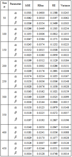
|
 under Type-I Censoring
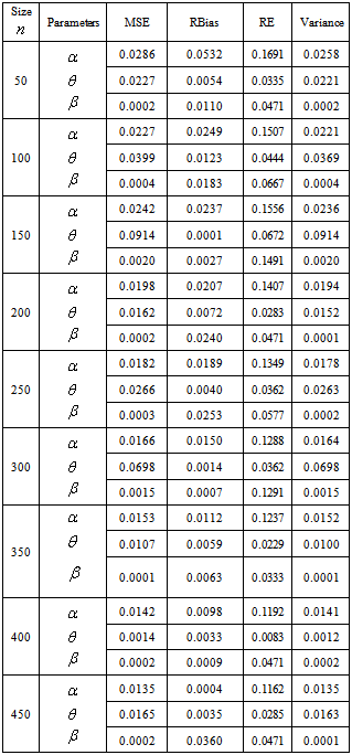
|
|