1. Introduction

Strategies for quick and accurate computation of Cumulative Distribution Functions (CDF) and more especially far quantiles is a topic common to a large variety of domains, such as finance, communications, insurance or nuclear physics[1][2], which led researchers to propose a collection of solutions more efficient than the “brute force” of Classical (or “Crude”) Monte-Carlo (CMC). The family of Importance Sampling (IS) strategies is certainly among the most efficient ones to achieve that[3], at least theoretically, since the ideal sampling scheme requires knowing the response (or even better: its density of probability) in order to adjust the sampling to it[1][3]. Indeed, blindly applying an IS strategy such as scaling or translation[3][4], exposes to the risk of getting an increasing variance instead of a decreasing variance of quantile estimates[5].

In the context of microelectronics circuit design, and more particularly semiconductor memories, of primary interest to us, there has been a growing interest in these computation-effective solutions over the past years[6 -9].

The fundamental reason lies in the growing impact of the various sources of statistical fluctuations of unit devices composing the memory cells as technologies progress [10-13] and in the rapid growth of memory capacity, now already entering the 10-100Gb era for standalone memories[14]. In the case of MOSFET transistors, for example, the threshold voltage fluctuation is a well known effect originating from multiple physical sources of randomness[13].

If not taken into account properly, these fluctuations are likely to degrade the overall design performance and ultimately compromise the functionality itself, if the failure rate exceeds a critical value (depending on the redundancy scheme used, in the case of memories[15]).

Classically, to assess memory design functionality towards cell fluctuations, CMC is performed and various critical signals of the circuit are analyzed (voltages, currents, delays, etc.). Since CMC is CPU intensive and practically ineffective in predicting far quantiles, it is not suitable for Giga-bit arrays. An ideal replacement strategy would not only show significant gain over CMC but be versatile enough to analyze multiple arbitrary signals in a single set of simulation runs, which does not fit well the classical IS strategies, where the sampling is adaptive to a response. Indeed, in the case of multiple responses, applying an IS strategy tuned for a given response to another one, the same above-mentioned risk of a diverging variance exists.

For this reason, we recently proposed[16][17] a more generic sampling strategy based on the enhancement of rare events – i.e. with a low probability of occurrence in the parameter space – suitable to any response and that does not require knowing the responses or even deciding beforehand which ones will be analyzed. The proposed method is called eXtreme Event Sampling (XES), as it favors the rare events that are significantly deviating from the nominal parameter conditions for which the circuit is expected to be in its ideal operation region. More specifically, a refined sampling is applied in selected probability ranges, which extends the CDF calculation of a response to far quantiles. In that sense, since XES enhances specific categories of events, it can be considered as an IS scheme and actually shows similar formulas, as we will expose in this article.

In a first section, we will detail the theoretical background supporting the construction of the sampling method, including the transformation allowing non-normal parameter distributions to be taken into account. In a second section, we will illustrate the effectiveness of XES through empirical studies for various responses, distributions and number of parameters and finally provide a benchmark of XES to CMC.

Definitions:

X_kⁱ : a vector of k i.i.d. random variables at iteration i

R(X_kⁱ): response (scalar) of a vector X_kⁱ

f(.): probability density function (PDF)

F(.): cumulative distribution function (CDF)

F^-1(.): inverse CDF

I(T): indicator function yielding 0 if T is false, 1 otherwise

N(µ,σ²): normal distribution of mean µ and variance σ²

ξ_p: p-quantile of a distribution = F^-1(p)

: estimator of ξ_p

W_i(.): i^th statistical weight of an IS run

N: total number of samples in MC or IS run

Φ(.): standard normal CDF

z: radius of a k-sphere

n(z): function yielding a number of samples per sphere

All random variables are assumed independent

2. Construction of the Sampling Method

2.1. The Multivariate Normal Distribution

The lack of information on the responses does not prevent calculating a probability of occurrence of events in a multivariate problem. The idea of XES is to do so in order to over-sample rare events and thus enhance the CDF calculation for far quantiles as compared to a CMC sampling. In order to identify such rare events, we first have to establish the joint probability of a set of random variables (x_k).

With the assumptions that all input variables are normally distributed and independent, the multivariate joint Probability Density Function (PDF) of a set x_k of such variables (x_k ~ N(µ_k,σ_k²)) reads[18]:

(1)

Iso-density curves for such a PDF are defined by assuming a constant exponential term as in (2), thus forming a family of parameterized ellipsoids[18] (see illustration for k=2 in Figure 1). The constant parameters z, µ_k and σ_k fully characterize the ellipsoid.

(2)

Applying a change of variable X_k = (x_k-µ_k)/σ_k, (2) now represents a hyper-sphere with respect to X_k in a space of dimension k (or k-sphere), and z is its radius. In the following, for the convenience of notations, we will always consider variables normalized to the standard N(0,1) distribution, unless otherwise specified. The choice of hyper-spherical coordinates to represent the samples is then the most natural one: the k Cartesian coordinates are represented by a radius z and (k-1) angles θ_i[19]:

(3)

Using such hyper-spherical coordinates (3) and normalized variables (or μ_k=0, σ_k=1), the PDF (1) now simply reads:

(4)

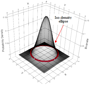Figure 1. Example of bivariate probability density function with an iso-density ellipse highlighted. X, Y ~ N(0,1). X/Y scales in standard sigma

As expected, since the hyper-spheres represent iso-density curves (radial symmetry of the density of probability), (4) shows no dependence to the (k-1) angles θ_i of the system.

As a consequence, calculating the CumulativeDistribution Function (CDF) from (4) using these coordinates can be done regardless of the angular position and with a single variable of integration: z. It also implies that a given k-sphere is not only an iso-density surface but also an iso-probability surface. Finally, since the variable z represents the distance from the center point of the parameter space (z=0 means all variables are at their average value), low probability events of interest for XES corresponds to high z values – this aspect is further commented in section 2.5, especially as regards the case of circuit analysis.

In the proposed technique, we take advantage of these properties to calculate the CDF of responses of multiple variables, using randomly chosen samples on concentric hyper-spheres and a modulation of the sampling versus the parameter z to enhance rare events in selected ranges of probability of occurrence.

We will now describe how to achieve such a sampling plan in practice and how to calculate the CDF of arbitrary responses.

2.2. Marginal PDF on k-Spheres

Let’s first establish the natural density of samples on a given k-sphere, by calculating the following marginal PDF (p_z) of events for a k-sphere of radius z:

(5)

where dV is the volume element (Jacobian) of the k-sphere. In the hyper-spherical coordinates, dV reads[19]:

(6)

Hence, we can rewrite the integral in (5):

(7)

with S_k being, by definition, the area of the unit k-sphere[20]:

(8)

As a result, p_z reads:

(9)

then, calculating the corresponding CDF from (9) requires integrating p_z with z varying from 0 to +∞.

2.3. Empirical CDF Calculation

Let’s now introduce a function n(z) yielding a number of samples n for a given k-sphere radius z. Since the natural density of samples for a given sphere z is defined by (9), the corrected marginal PDF for a such a sampling plan equals p_z/n(z). Taking into account the above and similarly to the classical Monte-Carlo technique[21], we can then compute the empirical probability F(ξ) for a response R(X_k) to be lower than ξ from the following discrete sum (in other words: the discrete CDF of R):

(10)

for a given series of radiuses z_i and a constant stepping dz, and with N being the total number of samples:

(11)

F(ξ) can also be written:

(12)

Such a formulation is similar to Importance Sampling techniques[3], W(z_i) representing the statistical weight associated to samples. In practice, the integration variable z is taken on a constant grid (dz constant), which also makes the integration method somewhat similar to a quasi-Monte-Carlo approach[21], but with a grid representing here equi-probable occurrences.

Theoretically, the sum of weights thus defined (12) should exactly equal one. In practice, however, discrete summation and numerical error lead to significant deviations from this ideal situation, which suggests performing a normalization of weights to their average, as often reported in the literature[3][22]:

(13)

This last formulation (13) is the selected method for all CDF calculations presented below.

Finally, it is easy to verify that if n(z_i) is chosen equal to p_z (9), then W(z_i)=1 hence (13) becomes a CMC sampling.

2.4. Uniform Sampling on k-Spheres

We implicitly assumed in the above reasoning that the n samples taken on a k-sphere of radius z were equi-probable. In order to respect this condition, we chose to use the following method, introduced by Marsaglia[23], to draw samples over a k-sphere with a uniform spatial distribution:

(14)

where (X_i) are the k Cartesian coordinates of the samples.

The k normally distributed samples are drawn, for example, by using the inverse normal CDF Φ^-1(u), with u being uniformly distributed over[0,1[. Alternatively, a low-discrepancy sequence or a stratification technique (such as Latin Hypercube Sampling – LHS)[21][24] can be used to draw the required u_k samples from the hyper-cube[0,1[^k. We briefly verified that the evenness of sample distribution over k-spheres was indeed improved using a LHS strategy (not illustrated here). In the rest of the article, we will assume that simple uniform random samples u_i and the inverse normal function Φ^-1(u_i) are used to generate the above X_i coordinates.

2.5. Sampling Plan: Defining n(z)

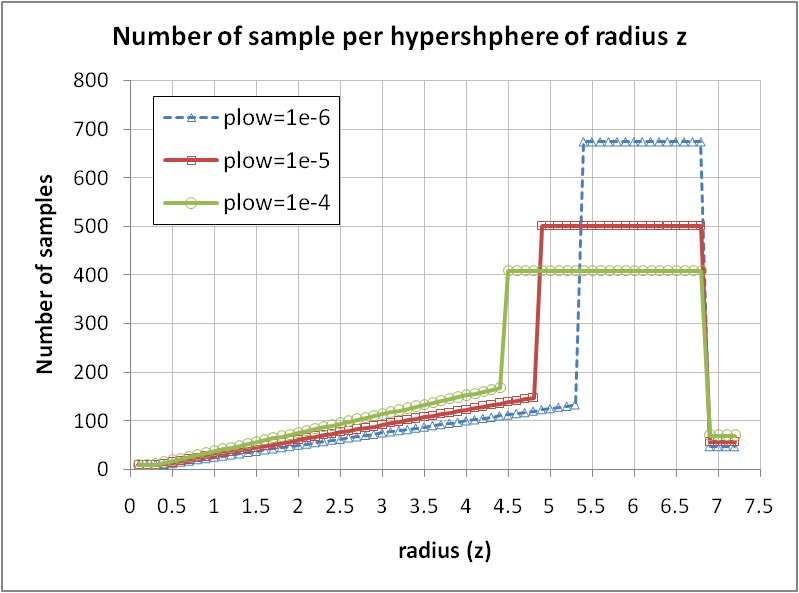
The last part of the method consists in choosing a number of samples per k-sphere for each radius z.

The primary goal of XES being to favor rare events in a selected range of occurrence probability, we first have to compute the CDF of events from the joint PDF (9). The PDF for various k values are illustrated in Figure 2, and (1-CDF) is shown in Figure 3.

We stress again here that this represents the probability of a set of events belonging to a given k-sphere to occur, regardless of the actual values of the response, since the response is assumed to be unknown at this stage.

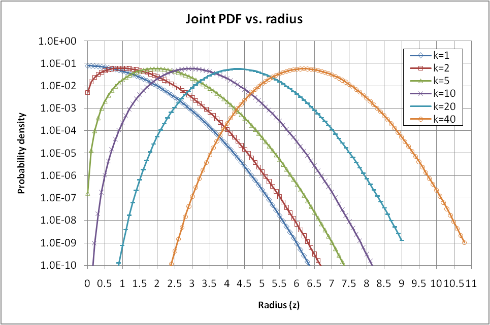Figure 2. Joint PDF (9) vs. radius z for various k. Y scale is in log

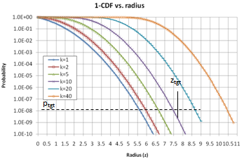Figure 3. (1-CDF) vs. radius z for various k. Y scale is in log

For a probability of interest p_tgt, for example, finding the corresponding radius z_tgt requires solving (15), as graphically illustrated in Figure 3:

(15)

For example, z_tgt approximately equals 7.8 for a targeted probability of 10^-9 and k=10 input variables (Figure 3).

This is the calculation used in XES to selectively refine the sampling in a range of radiuses corresponding to a range of probability of occurrence.

As in practice, we want to focus on given ranges of probability events far from the center of the parameter space (z=0), we will now design a sampling plan selectively enhancing the upper part of the CDF (15).

We underline here that, strictly speaking, low probability events can also happen at low radiuses for higher k values, as shown in Figure 2; these events are however very close to “nominal” conditions (i.e. all parameters at their average value for z=0) so are not really relevant to circuit analysis for which risks of functionality loss are expected for large deviations from typical conditions (high z values); note that it might not be the case in other particular contexts, in which low z values may contribute to lower and/or upper part of the CDF of the response and be the actual region of interest.

Using (15), lower and upper radiuses are calculated defining a region where the sampling refinement will be applied. Typically, the upper radius is taken at the lowest observable probability of occurrence in a given context (e.g. one over the number of cells in a memory array). In the following, the lower radius is varied depending on the objective of overall refinement of CDF or more selective refinement close to the upper radius, as illustrated in section 3.1. Outside of the refinement region, the sampling is relaxed. Optionally, the sampling can be extended beyond the upper radius (lowest probability of occurrence) in order to further refine the CDF near far quantiles.

As regards the evolution of the number of samples vs. radius, we chose a simple composition of linear growth and step functions. Other schemes are of course possible and would deserve a more in-depth investigation to determine an optimal n(z) function, particularly when k takes large values, since the area S_k (8) of k-spheres to be sampled grows rapidly with k (~z^k-1).

A typical sampling plan according to the above scheme is illustrated in Figure 4 in the case of 3 variables. The total number of samples is ~2.10⁴ in this example. The lower boundary of sampling refinement region (region 2) is set to z_low=3.7 (corresponding to p_low=0.005), the upper boundary to z_tgt=6.8 (p_tgt=10^-9). In this case, 3% of the total number of samples were allocated to sampling beyond this limit, up to p_high=p_tgt/10=10^-10 (region 3). The dz parameter is set to 0.1.

An illustration of XES as compared to CMC sampling is shown in Figure 5 in the case of 2 random variables (N(0,1)). The isotropic sampling refinement for outer circles is the basic property of such a sampling strategy: without information on the response, no direction of space is favored. In this example, the coverage of parameter space with XES is almost reversed as compared to CMC, which is a typical sampling that XES can provide to outperform CMC.

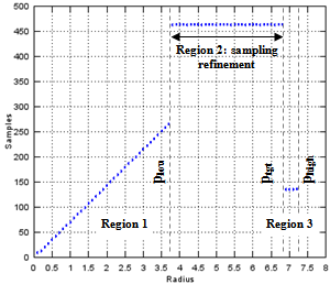Figure 4. Sampling plan for 3 variables for a targeted probability of 10-9. The lower boundary of sampling refinement corresponds to plow=0.005, the upper boundary corresponds to ptgt=10-9; over-sampling beyond this radius aims at improving the CDF estimation in the vicinity of the targeted probability. The maximum radius corresponds to phigh=10-10. dz=0.1

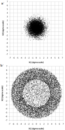Figure 5. Illustration of sampling plans for 2 random normal variables N(0,1) for a/ CMC b/ XES strategies. Both cases have 10,000 samples. Targeted probability is ptgt=10-9, lower refinement boundary is plow=10-3. Scales are in sigma of the standard normal distribution

2.6. Actual Coordinates and Non-Normal Distributions

Up to this point, the random variables are still expressed in a standard normal scale. Therefore, for each variable, a transformation of coordinates from the standard normal distribution to their actual distribution has to be performed before acquiring (or simulating) the responses. For a normal distribution, this is simply achieved by restoring the proper standard deviation (σ) and mean (µ) along the k axes:

(16)

For non-normal distributions D, the inverse transform method[25] is applied to the relevant coordinates x_i:

(17)

Figure 6 illustrates how the sampling plan is modified by such a transformation for a normal distribution (along the horizontal axis) and a Weibull distribution (along the vertical axis) from the 2D sampling plan illustrated in Figure 5. The iso-probability contours are preserved by this transformation. As a result, in the example of Figure 6, it tends to concentrate more samples in the lower part of the space, due to the Weibull distribution shape (more visible in logarithmic scale). Within the XES strategy, this property ensures an even sampling, probability-wise, throughout the parameter space. However, the initial uniformity of samples on the k-spheres is not preserved by transformations (16) and (17), so the mean distance between samples on the new iso-probability surfaces is now varying (visible on the graph a/ of Figure 6), which tends to favor some portions of the space for a given probability of occurrence (no bias introduced, but coverage of space degraded). Searching a correction function to compensate for this modulation of density and thus further improve XES is certainly a topic of interest, but is however well beyond the frame of this work.

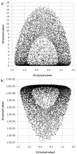Figure 6. 2D sampling plan of Figure 5 after transformation of coordinates; X1: N(0,0.35²); X2: Weibull (scale=2,shape=1.5). a/ linear Y-scale; b/ logarithmic Y-scale

Finally, we stress here that the sampling itself is independent from the coordinate transformation (16) and (17). It implies that a same sampling plan can also potentially be used for various parameter distributions, which is of interest for example in a “what-if” analysis: studying the impact of changing the standard deviation of one of the variables does not require regenerating the sampling plan.

2.7. Confidence Interval, Error Calculation and Gains

To calculate a confidence interval (CI) on the estimated quantile ξ_p, we use the classical property of convergence in distribution of quantile error, as described in e.g.[26]:

(18)

where ψ_p is the standard deviation of the probability p (non-normalized to N) and f(ξ_p) is the PDF of the response at the p-quantile, estimated in the following from the empirical CDF using a finite difference estimator as proposed in[26].

In the case of IS, the best estimator of the empirical variance ψ² depends on p and reads[26]:

(19)

For CMC, the asymptotic value of ψ² reads[26]:

(20)

From (18), the standard deviation of the p-quantile estimator (ξ_p) reads:

(21)

where ψ_p is calculated from (19) for XES or (20) for CMC.

Then, to calculate a 95% CI, we used the classical approximation:

(22)

In order to estimate the accuracy of estimated probabilities, we also calculate the relative error ε_p on a given probability p[1]:

(23)

To further check the validity of the above confidence interval estimate (22) in the case of XES, we experimentally compared it to a CI calculated by re-sampling through a bootstrap (BS) technique and using Studentized statistics [27][28]. As we will illustrate in the next section, a good agreement is observed between the CIs calculated by the two methods.

Finally, we define two gains (Ga, Gs) to measure the performance of XES over CMC:

(24)

G_a being the gain in accuracy at a given sampling N, and G_s the gain in sampling at a given relative error ε_p (15% in this case). We can notice that the gain Ga is the ratio of relative errors, which is actually equivalent to a classical metric measuring the gain of an IS over CMC at a given p-quantile for a constant number of samples N: Ga~σ_MC/σ_IS[4].

3. Empirical Study

We implemented the above formulas and sampling scheme in a commercial numerical computing platform in order to evaluate the accuracy and efficiency of the XES method, as we will now illustrate. The examples shown hereafter are built around a series of simple electrical test circuits made of resistors connected in series or in parallel and biased under a constant current Ic (Figure 7). The studied response is a voltage drop (Vd) across the circuit, and the random variables are the resistances. These simple circuits could represent, for example, a memory cell that would be repeated over a memory array and would experience statistical variations of its parameters (here: the resistance value).

Since the equivalent resistance of such circuits is calculable, the response has a known analytical formula (Figure 7). In the following examples, this formula is used to calculate the response Vd for each sample and hence reconstruct the CDF; in an actual implementation, a circuit solver would compute the responses.

Notes: probabilities in the CDF graphs below are expressed in sigma of the standard normal distribution, except otherwise specified. On such a scale, purely normal distributions show up as a straight line. The parameter dz in (12) is set to a constant value of 0.1 in all the examples below.

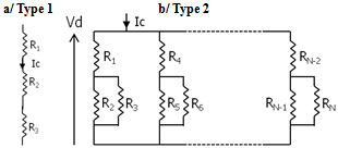Figure 7. Test circuit schematics with resistors in a/ series (s) (Type 1) or b/ series (s) and parallel (//) (Type 2). The equivalent resistance Req can be calculated in all cases using the classical formulas Req(Rx.s.Ry)=Rx+Ry Req(Rx//Ry)=Rx.Ry/(Rx+Ry). The studied response is the voltage drop Vd across the group of resistors under a constant current Ic (Ic=1mA in all the following examples): Vd=Req Ic

3.1. Linear Response

We will first illustrate XES in the case of a Type 1 circuit (Figure 7 a/) for which the response is linear with respect to the resistances, and for 3 resistors: R1, R2, R3, following normal (section 3.1.1.) or non-normal (section 3.1.2.) distributions.

3.1.1. Normal Distributions

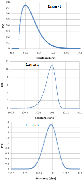
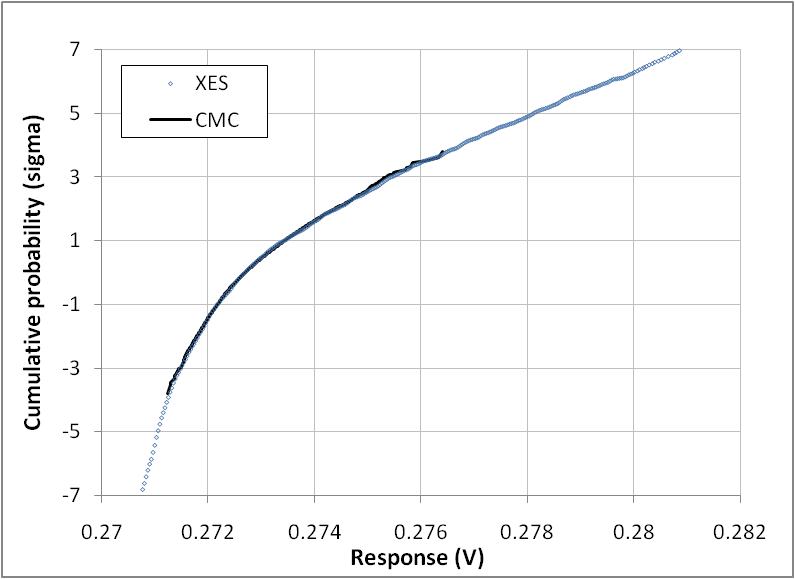
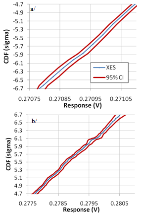
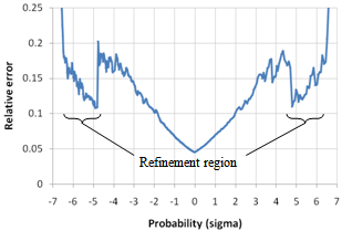
The resistors are chosen as follows: R1:N(50,0.5²); R2: N(100,10²); R3:N(120,1.5²) – all values in ohm. The number of samples was set to 13,896 for the various plots below.

Figure 8 shows the resulting XES CDF for Vd with the p_low parameter set to 10^-6 and for a targeted probability of 10^-9 (assuming the studied population is of 1 billion individuals). Since in this case, the theoretical CDF can also be calculated from the composition of variance[18], we also plotted it in the same graph, in order to check that the two traces were superimposed.

The 95% CI was also computed and is shown in Figure 9 together with the CDF for the lower (a/) and upper (b/) part of the CDF. The CI calculated with (22) and from a bootstrap re-sampling gives consistent results. As expected, thanks to the XES strategy, the CI is narrow in the vicinity of the targeted probability, both at +6σ and at -6σ.

The relative error on the estimated quantiles (δξ) can also be calculated in this specific case, since the theoretical CDF and hence the true ξ_p are known:

(25)

With the above sampling plan, the measured δξ at ±6σ is well below 1% (typically around 0.1-0.2%).

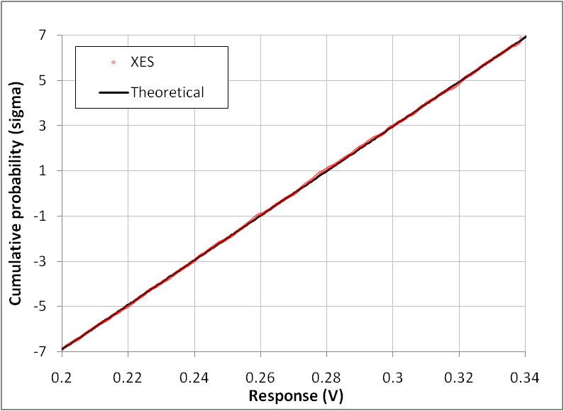Figure 8. CDF (sigma scale) of voltage drop (Vd) for 3 resistors / Type 1 circuit. The ptgt parameter is set to 10-9 and plow to 10-6. XES CDF is superimposed to the theoretical straight line

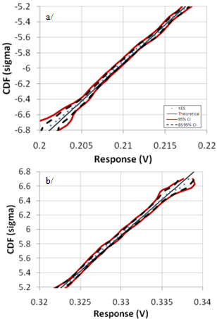Figure 9. Detail of a/ lower and b/ upper part of the XES CDF of Vd from Figure 8 as compared to the theoretical straight line; 95% CI calculated from (22) or from BS re-sampling (1000 runs)

The effect of modulating the refinement region (Figure 10) through the p_low parameter at a constant number of samples on the error ε_p is illustrated in Figure 11. The peak relative error observed in the 4-5σ range tends to decrease and to shift to lower σ for increasing p_low, while the relative error degrades at the targeted probability of ±6σ. In this example, the criterion of ε_p < 15% at ±6σ is reached for plow=10^-6.

Another property of XES is evidenced in Figure 11: because of the symmetry of the sampling on k-spheres, both ends of the CDF are refined by over-sampling rare events corresponding to large z radiuses, leading to an accurate estimation of p_tgt (-6σ) and 1-p_tgt (+6σ) together. This is a key feature to analyze responses showing a two-sided operating range (i.e. both low and high values leading to circuit failure). As already mentioned before, we exclude from this study the particular cases of responses exhibiting far quantiles at low z-values (specific non-monotonic functions), for which the above sampling refinement would not be effective on the lower (or upper) side of the CDF.

Figure 10. Sampling plan for various plow, at a constant N=13,896

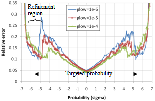Figure 11. Relative error εp vs. probability for various plow values at a constant N for CDF of Figure 8. The variations of plow modulate the refinement sampling range and the accuracy in this region

3.1.2. Non-Normal Distributions

In this example, the circuit is identical to the previous (3 resistors in series) and resistances are simply changed to 3-parameter Weibull (W) distributions instead of normal, as follows: W_R1(scale=1, shape=1.5, location=50), W_R2(scale= 1, shape=30, location= 100), W_R3(scale=1, shape=4.5, location=120). The values were chosen to yield various PDF asymmetries, as illustrated in Figure 12. The XES parameters are: N=13,872 samples, p_tgt=10^-9, p_low=10^-4. The resulting XES CDF is shown in Figure 13 and is superimposed to the CMC trace. The confidence interval in the lower and upper part of the CDF are shown in Figure 14, further illustrating the good accuracy obtained at extreme quantiles even for non normal distributions.

Figure 12. PDF of the resistances R1, R2 and R3 (Weibull distributions)

Figure 13. XES and CMC CDF of the response Vd of 3 resistances following 3-parameter Weibull distributions, Type 1 circuit

Figure 14. XES CDF of Vd and 95% Confidence Interval from (22) for a/ lower and b/ upper part of the CDF

3.2. Non Linear Response

Considering now a Type 2 circuit and three normally distributed resistances, the resulting response Vd is non-linear, due to the resistors in parallel (Figure 7). In the following example, the resistances are chosen identical to the ones of section 3.1.1. The sampling plan is also similar, with p_tgt=10^-9, p_low=10^-5 and N=13,880 samples. The CDF of the response are shown in Figure 15 together with the 95% CI calculated from (22) or with 1000 BS runs. Tight CIs are obtained in the targeted probability range and the two CIs are consistent.

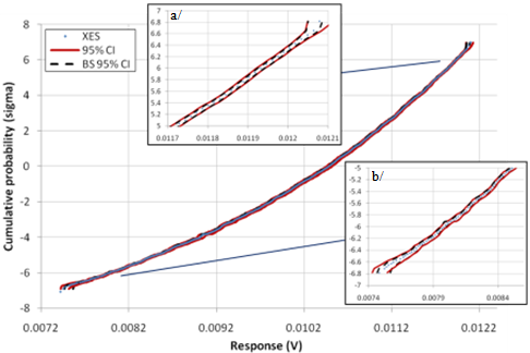Figure 15. XES CDF of Vd and 95% confidence interval from (22) and from BS using 1000 runs (insets: detail of the a/ upper and b/ lower part of the CDF). Type 2 circuit with 3 resistors identical to section 3.1.1

Figure 16. Relative error εp vs. cumulative probability (sigma scale)

Finally, the relative error (ε_p) curve shown in Figure 16 clearly demonstrates the effect of the sampling refinement on the accuracy and illustrates that ε_p~15% at p_tgt=10^-9 is reached for these sampling conditions, hence proving the effectiveness of XES also for non linear responses.

3.3. Multiple Responses, Single Sampling Plan

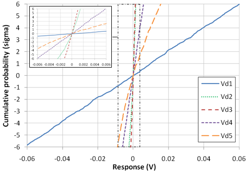Figure 17. CDF of various responses, single sampling plan, plow, =10-4, N=13,989. The responses have been normalized (shifted to their median) in order to represent the various responses on the same x-scale

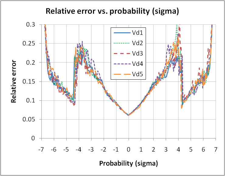Figure 18. Relative error εp for the various responses Vd1 to Vd5, single sampling plan, plow, =10-4, ptgt=10-9, N=13,989

In cases where the response has a known analytical formula as in the above examples, IS approaches such as exponential twisting[29] or mixture IS[8], for example, would certainly be more efficient, but restricted to one response at a time, as the sampling is adjusted to the response shape (either by knowing the response beforehand, or through a feedback of the response on the sampling while running). On the contrary, XES is built to deal with multiple arbitrary responses with a single set of samples, as we will now further illustrate on an example.

Let’s consider 5 different responses of 3 normally distributed variables, built as follows: Vd1 is a linear response (Type 1 circuit) identical to section 3.1.1. Vd2 is identical to section 3.2 (Type 2 circuit), Vd3 and Vd4 are also from a Type 2 circuit but with a cyclic permutation of resistances as compared to Vd2. Vd5 is a purely fake response, built from the sum of square of resistances multiplied by a constant (10^-6), in order to illustrate the case of a response that is non linear and non-monotonic with respect to all its variables.

As shown in Figure 17, despite the collection of responses yielding a large variety of CDF shapes, XES allows calculating all of them from a single set of samples. Moreover, in the sampling refinement region (p_low=10^-4 ; p_tgt=10^-9), the relative error ε_p is low and is similar for the various responses, as illustrated in Figure 18, proving the effectiveness and robustness of the method to arbitrary response shapes.

3.4. Larger Number of Variables (k)

As mentioned in section 2.5, the area of a k-sphere is growing rapidly with k and z, hence the number of samples required by XES is expected to grow accordingly for far quantiles.

We have empirically studied the evolution of the minimal sampling to reach a given relative error (ε_p<15%) at a target quantile (for both p_tgt and its counterpart 1-p_tgt), using a simple response (Type 1 circuit) and a growing number of normally distributed variables (k). As graphically illustrated in Figure 19 for two target quantiles (p_tgt=10^-9 and 10^-10), the growth of the number of samples vs. k is indeed fast, especially in the initial range of 3-12 variables.

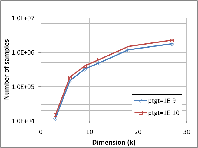Figure 19. Required number of samples to reach εp<15%@ptgt vs. number of variables (k) for two target quantiles, 10-9 and 10-10. Response is Vd of a Type 1 Circuit; all variables are normally distributed

Figure 20. XES and CMC CDF of a response (Vd) of 18 variables; Type 2 circuit with resistance mean ∈[50 100 120 60 130 90 70 110 150 140 80 110 105 70 90 85 108 160] and standard deviation ∈[0.5 10 1.5 0.7 10 3.5 0.5 3 5.5 5.5 3 2.8 7.8 1.8 2.2 5 9 3]. 95% CI calculated from (22). ptgt= 10-9 plow=10-3, N=1.4.106 samples

We also verified that a CDF of a non linear response (Type 2 circuit) could also be computed with a reasonable accuracy in similar sampling conditions, as illustrated in Figure 20 for 18 variables. In this example, the sampling is optimized to keep a tight CI over the full CDF rather than yielding a given accuracy for a given quantile.

3.5. Benchmark to CMC

Based on the previous results, we will now further illustrate the efficiency of XES as k grows by comparing its performances to CMC in term of gain in sampling (Gs) and in accuracy (Ga) as defined in (24).

The Tables 1 and 2 below show the gains obtained for p_tgt=10^-9 and 10^-10, respectively, and for various k (up to k=27), considering a response Vd from a Type 1 circuit. The same data are graphically illustrated in Figure 21 and 22, showing that both gains stay quite strong even for 27 variables and further grow as the target quantile is decreasing to p_tgt=10^-10. It also shows that the gain degradation tends to attenuate as k grows, suggesting that the efficiency of XES over CMC should stay significant for an even larger number of variables.

We finally underline that the error on the estimated quantile δξ at p_tgt was below 1% for all the XES results of Tables 1 and 2, proving that the method does not introduce significant biases in the far quantile estimates.

Table 1. Expected gains as compared to CMC – various plow, ptgt=10-9 k Sampling (N) Gain vs. CMC at ptgt=10-9 Gs: sampling gain at 15% relative error on ptgt Ga: accuracy gain at given sampling 3 1.2E+04 4.2E+06 1924.5 6 1.5E+05 3.3E+05 544.3 9 3.30E+05 1.5E+05 367.0 12 5.0E+05 1.0E+05 298.1 18 1.2E+06 4.2E+04 210.8 27 1.8E+06 2.8E+04 157.1

Table 2. Expected gains as compared to CMC – various plow, ptgt=10-10 k Sampling (N) Gain vs. CMC at ptgt=10-10 Gs: sampling gain at 15% relative error on ptgt Ga: accuracy gain at given sampling 3 1.5E+04 3.3E+07 5443.3 6 1.9E+05 2.6E+06 1529.4 9 4.10E+05 1.2E+06 1041.2 12 6.3E+05 7.9E+05 839.9 18 1.5E+06 3.3E+05 544.3 27 2.30E+06 2.2E+05 439.6

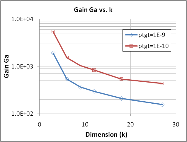Figure 21. Gain in accuracy of XES over CMC vs. k for two target quantiles ptgt=10-9 and 10-10 and at a given sampling (see Tables 1 and 2). Response is Vd of a Type 1 Circuit; all variables are normally distributed

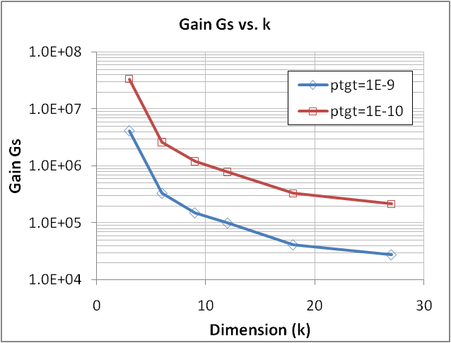Figure 22. Gain in sampling of XES over CMC vs. k for two target quantiles ptgt=10-9 and 10-10 and for εp<15%. Response is Vd of a Type 1 Circuit; all variables are normally distributed

4. Conclusions

We propose a multivariate sampling method, called XES (eXtreme Event Sampling), as an alternative to CMC and classical IS to compute far quantiles of arbitrary responses. The proposed strategy is similar to an IS scheme, but unlike classical IS techniques, does not require to know the response in advance or to adjust the sampling plan to it. Instead, events of low probability of occurrence are over-sampled in order to enhance far quantiles of responses.

As a result, CDF of arbitrary responses can be reconstructed with a good accuracy at extreme quantiles and much more efficiently than CMC, despite the fact the method is generic as compared to an IS approach.

The method applies to normally or non-normally distributed parameters and can deal with a large number of variables (up to 27 tested).

Thanks to its flexibility, we believe XES is a valuable alternative to classical IS strategies when multiple arbitrary responses are to be studied in a single-pass simulation run (i.e. without adapting the sampling from the responses). Thus, beyond the case of circuit design of interest to us, the method could apply to other domains showing similar constraints.

Future developments of the method should include in-depth investigation of the optimal sampling strategy (n(z) function) vs. k, further benchmark including to other IS strategies and finally, implementation of XES in a circuit solver to study real cases.

ACKNOWLEDGEMENTS

The authors would like to acknowledge Alessandro Calderoni and Andrea Marmiroli (Micron Technology Italy) for their kind support and for valuable discussions and suggestions during the development of the XES method.