1. Introduction

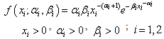
The Gumbel type II distribution is used to model the extreme events like extreme earthquake, rainfalls, temperature, floods etc. It has another side of applications which deals with life testing experiments. Chechile[1] obtained the posterior distribution assuming that the random sample is taken from the Gumbel distribution using the conjugate prior. Corsini et al.[2] discussed the maximum likelihood (ML) algorithms and Cramer-Rao (CR) bounds for the location and scale parameters of the Gumbel distribution. Mousa[3] obtained the Bayesian estimation for the two parameters of the Gumbel distribution based on record values. Koutsoyiannis and Baloutsos[4] described that the Gumbel distribution has been the prevailing model for quantifying risk associated with extreme rainfall. Rasmussen and Gautam[5] extended the probability weighted moments (PWM) to what is called the generalized method of probability weighted moments (GPWM) because there is no reason why the PWMs provide the most efficient estimators of Gumbel parameters and quantile especially in hydrology. Malinowska and Szynal[6] obtained the Bayes estimators for the two parameters of a Gumbel distribution based on kth lower record values. Nadarajah and Kotz[7] introduced the beta Gumbel (BG) distribution and provided closed-form expressions for the moments, the asymptotic distribution of the extreme order statistics and discussed the maximum likelihood estimation procedure. Miladinovic and Tsokos[8] modified the classical Gumbel probability distribution in order to study the failure times of a given system. Park et al.[9] gave a novel equation for the scale parameter of the Gumbel distribution. Heo and Salas[10] examined the log-Gumbel distribution regarding quantile estimation and confidence intervals of quantiles. Thompson et al.[11] introduced a distributional hypothesis test for left censored Gumbel observations based on the probability plot correlation coefficient (PPCC).

The mixture models have received great attention of the analysts in the recent era. These models include finite and infinite number of components that can analyze different datasets. A finite mixture of probability distribution is suitable to study a population categorized in number of subpopulations. A population of lifetimes of certain electrical elements can be classified into number of subpopulations based on causes of failures. The analysis of mixture models under Bayesian framework has developed a significant interest among the statisticians. The authors dealing with Bayesian analysis of mixture models include Saleem and Aslam[12], Saleem et al.[13], Majeed and Aslam[14] and Kazmi et al.[15]. These contributions to the mixture models are the great motivations for the resent study.

We considered two component mixture of Gumbel type II distribution. The population of certain items is assumed to be partitioned into two subpopulations. The randomly selected observations from the said population are considered to be a part of one of the above mentioned subpopulations. These subpopulations are assumed to follow the Gumbel type II distribution. Therefore, the two components mixture of Gumbel type II distributions has been proposed to model this population. The observations have been assumed to be right censored. The inverse transformation technique of simulation under a probabilistic mixing has been used to generate data and to evaluate the performance of different estimators.

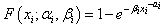
2. The Model and Likelihood Function

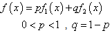
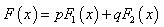
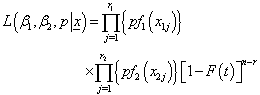
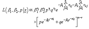
A density function for mixture of two components densities with mixing weights (p,q) is:

(1)

The following Gumbel type II distribution is considered for both mixture densities:

(2)

With the cumulative distribution function as:

(3)

The cumulative distribution function for the mixture model is:

(4)

Suppose n items are put on a life testing experiment and r units failed until time T while, n – r units are still working. Now based on causes of failure, the failed items are assumed to come either from subpopulation 1 or from subpopulation 2. Therefore it can be observed that r₁ and r₂ failed items come from first and second subpopulation respectively. Where r = r₁ + r₂. The remaining n – r items are assumed to be censored observations. The likelihood function for above censored data can be obtained as:

(5)

(6)

Expanding the last term by binomial expansion the likelihood function becomes:

(7)

Where

and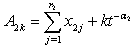

3. The Posterior Analysis under the Assumption of Uniform Prior

One of the most widely used non-informative priors, proposed by Laplace[16], is a uniform prior. It has been applied to many problems, and often the results are entirely satisfactory. This prior has been used for the posterior estimation.

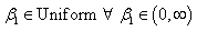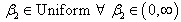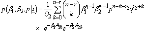
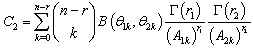
Let , and. Assuming independence, these priors result into a joint prior that is proportional to a constant. That joint prior has been used to derive the joint posterior distribution of . The marginal distribution for each parameter can be obtained by integrating the joint posterior distribution with respect to nuisance parameters. The joint posterior distribution is:

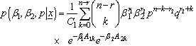(8)

Where

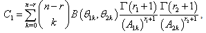
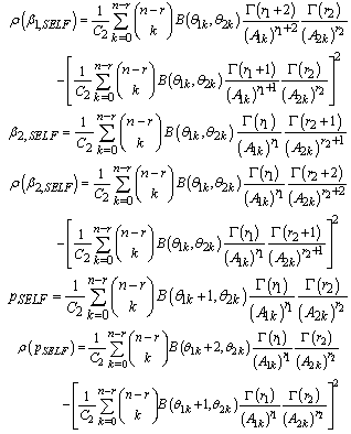
Using the posterior distribution, discussed in (8), the Bayes estimators and posterior risks under different loss functions have been derived and presented in the following.

Bayes estimators and associated risks under uniform prior using squared error loss function (SELF) are:

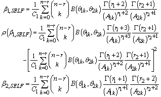
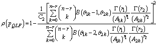
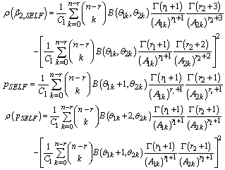Bayes estimators and risk under uniform prior using quadratic loss function (QLF) are:

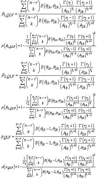Bayes estimators and risk under uniform prior using weighted loss function (WLF) are:

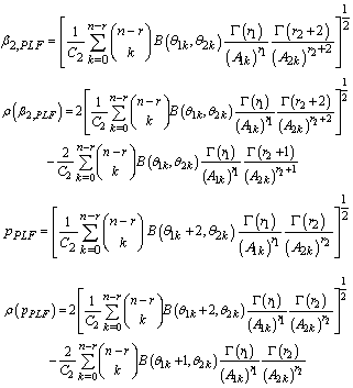
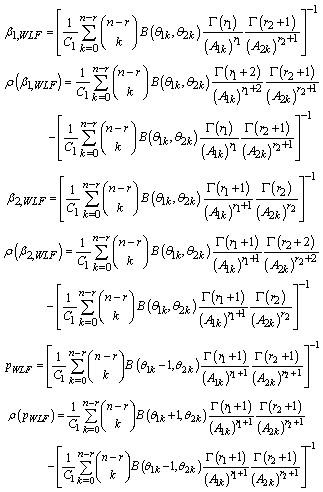Bayes estimators and risk under uniform prior using precautionary loss function (PLF) are:

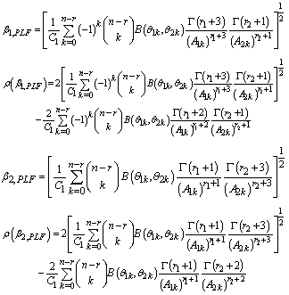
4. The Posterior Analysis under the Assumption of Jeffreys Prior

Another non-informative prior has been suggested by Jeffreys[17] which is frequently used in situations where one does not have much information about the parameters. This is defined as the distribution of the parameters proportional to the square root of the determinants of the Fisher information matrix i.e.

Where is the vector of parameters and is (2×2) Fisher information matrix, defined as;

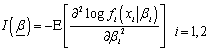Where have been defined in (2) and. Assuming independence, the joint prior is obtained as:

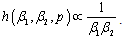(9)

The joint posterior distribution using the above prior is:

(10)

Where

The Bayes estimators and associated posterior risks have been derived under different loss functions using the posterior distribution (10).

Bayes estimators and associated risks under Jeffreys prior using squared error loss function (SELF) are:

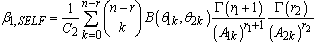
Bayes estimators and risk under Jeffreys prior using quadratic loss function (QLF) are:

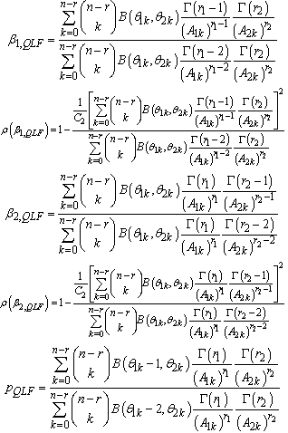
Bayes estimators and risk under Jeffreys prior using weighted loss function (WLF) are:

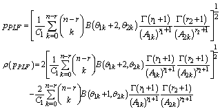
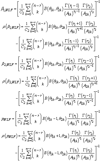Bayes estimators and risk under Jeffreys prior using precautionary loss function (PLF) are:

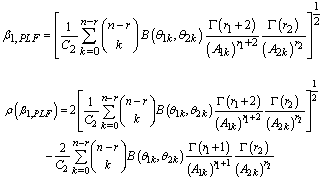
5. Posterior Predictive Distributions and Intervals

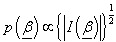
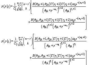
The posterior predictive distributions under uniform and Jeffreys priors are:

The posterior predictive intervals under uniform prior can be obtained by solving the following two equations respectively.

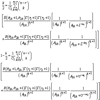Where ‘k’ is level of significance

The posterior predictive intervals under uniform prior can be obtained by solving the following two equations respectively.

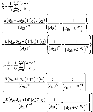
6. Simulation Study

A simulation study has been conducted to assess and compare the performance of Bayes estimators and to analyse the impact of sample size, mixing weight and magnitude of parametric values on the Bayes estimators. Samples of sizes n = 100, 200, 300, 400 and 500 have been generated by inverse transformation method from two components mixture of Gumbel type II distribution. The parametric values used are: 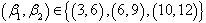and 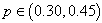. The probabilistic mixing has been used to generate the mixture data. For each observation a random number has been generated from . If the observation has been randomly taken from first subpopulation and if then the observation have been taken from the second subpopulation.

The observations above a fixed censoring time T have been assumed to be right censored. Under each combination of parametric values, the choice of censoring time has been made so that the censoring rate in the respective sample has been 20%. As one sample cannot completely describe the behaviour and properties of the Bayes estimators, the results have been replicated 1000 times and the average of results has been presented in the tables below.

Table 1. Bayes estimates and posterior risks under uniform prior using β1 = 3, β2 = 6 and p = 0.30 n β1 = 3 SELF QLF WLF PLF 100 3.28620 3.22048 3.25301 3.30310 0.05344 0.00270 0.01195 0.01216 200 3.26174 3.22912 3.24535 3.27001 0.02592 0.00135 0.00590 0.00595 300 3.19922 3.18322 3.19120 3.20324 0.01237 0.00068 0.00289 0.00290 400 3.10967 3.09931 3.10448 3.11228 0.00777 0.00045 0.00187 0.00187 500 3.03695 3.02936 3.03315 3.03886 0.00555 0.00034 0.00137 0.00137 n β2 = 6 SELF QLF WLF PLF 100 6.56364 6.43237 6.49734 6.59739 0.06136 0.00310 0.01372 0.01397 200 6.51478 6.44963 6.48204 6.53130 0.02976 0.00155 0.00677 0.00683 300 6.38990 6.35795 6.37389 6.39794 0.01421 0.00078 0.00331 0.00333 400 6.21105 6.19035 6.20068 6.21625 0.00893 0.00052 0.00215 0.00215 500 6.06581 6.05064 6.05821 6.06961 0.00638 0.00039 0.00157 0.00157 n p = 0.30 SELF QLF WLF PLF 100 0.33300 0.32634 0.32964 0.33471 0.00297 0.00015 0.00066 0.00068 200 0.33052 0.32722 0.32886 0.33136 0.00144 0.00008 0.00033 0.00033 300 0.32419 0.32257 0.32337 0.32460 0.00069 0.00004 0.00016 0.00016 400 0.31511 0.31406 0.31459 0.31538 0.00043 0.00003 0.00010 0.00010 500 0.30774 0.30698 0.30736 0.30794 0.00031 0.00002 0.00008 0.00008

Table 2. Bayes estimates and posterior risks under uniform prior using β1 = 3, β2 = 6 and p = 0.45 n β1 = 3 SELF QLF WLF PLF 100 3.26977 3.20438 3.23674 3.28658 0.05237 0.00265 0.01171 0.01192 200 3.24543 3.21298 3.22912 3.25366 0.02540 0.00132 0.00578 0.00583 300 3.18322 3.16730 3.17524 3.18723 0.01213 0.00066 0.00283 0.00284 400 3.09412 3.08381 3.08896 3.09671 0.00762 0.00044 0.00183 0.00184 500 3.02177 3.01421 3.01799 3.02366 0.00544 0.00033 0.00134 0.00134 n β2 = 6 SELF QLF WLF PLF 100 6.69491 6.56101 6.62729 6.72933 0.06258 0.00316 0.01399 0.01425 200 6.64508 6.57863 6.61168 6.66192 0.03036 0.00158 0.00691 0.00697 300 6.51770 6.48511 6.50136 6.52590 0.01449 0.00079 0.00338 0.00340 400 6.33527 6.31415 6.32470 6.34058 0.00911 0.00053 0.00219 0.00220 500 6.18712 6.17165 6.17938 6.19100 0.00651 0.00040 0.00160 0.00161 n p = 0.45 SELF QLF WLF PLF 100 0.49284 0.48299 0.48786 0.49538 0.00413 0.00021 0.00092 0.00094 200 0.48917 0.48428 0.48672 0.49041 0.00200 0.00010 0.00046 0.00046 300 0.47980 0.47740 0.47859 0.48040 0.00096 0.00005 0.00022 0.00022 400 0.46637 0.46481 0.46559 0.46676 0.00060 0.00003 0.00014 0.00014 500 0.45546 0.45432 0.45489 0.45575 0.00043 0.00003 0.00011 0.00011

Table 3. Bayes estimates and posterior risks under Jeffreys prior using β1 = 3, β2 = 6 and p = 0.30 n β1 = 3 SELF QLF WLF PLF 100 3.26429 3.19901 3.23132 3.28108 0.05245 0.00265 0.01173 0.01194 200 3.23999 3.20759 3.22371 3.24821 0.02544 0.00133 0.00579 0.00584 300 3.17789 3.16200 3.16992 3.18189 0.01215 0.00066 0.00283 0.00285 400 3.08894 3.07864 3.08378 3.09153 0.00763 0.00044 0.00183 0.00184 500 3.01671 3.00916 3.01293 3.01860 0.00545 0.00033 0.00134 0.00135 n β2 = 6 SELF QLF WLF PLF 100 6.55488 6.42378 6.48867 6.58858 0.06037 0.00305 0.01350 0.01374 200 6.50608 6.44102 6.47339 6.52258 0.02928 0.00153 0.00667 0.00672 300 6.38137 6.34946 6.36538 6.38940 0.01398 0.00076 0.00326 0.00328 400 6.20276 6.18208 6.19240 6.20795 0.00878 0.00051 0.00211 0.00212 500 6.05771 6.04256 6.05013 6.06151 0.00627 0.00038 0.00155 0.00155 n p = 0.30 SELF QLF WLF PLF 100 0.33081 0.32419 0.32747 0.33251 0.00287 0.00015 0.00064 0.00065 200 0.32835 0.32506 0.32670 0.32918 0.00139 0.00007 0.00032 0.00032 300 0.32205 0.32044 0.32125 0.32246 0.00066 0.00004 0.00016 0.00016 400 0.31304 0.31200 0.31252 0.31330 0.00042 0.00002 0.00010 0.00010 500 0.30572 0.30496 0.30534 0.30591 0.00030 0.00002 0.00007 0.00007

Table 4. Bayes estimates and posterior risks under Jeffreys prior using β1 = 3, β2 = 6 and p = 0.45 n β1 = 3 SELF QLF WLF PLF 100 3.24797 3.18301 3.21516 3.26467 0.05140 0.00260 0.01149 0.01170 200 3.22379 3.19156 3.20759 3.23197 0.02493 0.00130 0.00568 0.00573 300 3.16200 3.14619 3.15407 3.16598 0.01190 0.00065 0.00278 0.00279 400 3.07350 3.06325 3.06836 3.07607 0.00748 0.00043 0.00180 0.00180 500 3.00162 2.99412 2.99787 3.00351 0.00534 0.00032 0.00132 0.00132 n β2 = 6 SELF QLF WLF PLF 100 6.68597 6.55225 6.61844 6.72035 0.06157 0.00311 0.01377 0.01402 200 6.63620 6.56984 6.60286 6.65303 0.02987 0.00156 0.00680 0.00686 300 6.50900 6.47645 6.49268 6.51719 0.01426 0.00078 0.00333 0.00334 400 6.32681 6.30572 6.31625 6.33211 0.00896 0.00052 0.00215 0.00216 500 6.17886 6.16341 6.17113 6.18274 0.00640 0.00039 0.00158 0.00158 n p = 0.45 SELF QLF WLF PLF 100 0.48960 0.47981 0.48465 0.49212 0.00399 0.00020 0.00089 0.00091 200 0.48596 0.48110 0.48351 0.48719 0.00194 0.00010 0.00044 0.00044 300 0.47664 0.47426 0.47545 0.47724 0.00092 0.00005 0.00022 0.00022 400 0.46330 0.46176 0.46253 0.46369 0.00058 0.00003 0.00014 0.00014 500 0.45247 0.45133 0.45190 0.45275 0.00041 0.00003 0.00010 0.00010

Table 5. Bayes estimates and posterior risks under uniform prior using β1 = 6, β2 = 9 and p = 0.45 n β1 = 6 SELF QLF WLF PLF 100 6.21328 6.15114 6.18205 6.22903 0.06556 0.01495 0.03122 0.03150 200 6.11691 6.08633 6.10158 6.12461 0.03153 0.00747 0.01533 0.01540 300 6.06531 6.04509 6.05519 6.07039 0.02062 0.00498 0.01013 0.01016 400 6.07220 6.05702 6.06460 6.07600 0.01548 0.00374 0.00760 0.00762 500 5.97946 5.96750 5.97347 5.98246 0.01200 0.00299 0.00599 0.00600 n β2 = 9 SELF QLF WLF PLF 100 9.73303 9.63570 9.68412 9.75770 0.21487 0.01119 0.04891 0.04934 200 9.54646 9.49873 9.52253 9.55847 0.10257 0.00560 0.02393 0.02403 300 9.27926 9.24833 9.26377 9.28703 0.06445 0.00373 0.01549 0.01554 400 9.06227 9.03961 9.05092 9.06795 0.04604 0.00280 0.01134 0.01137 500 9.00161 8.98361 8.99260 9.00613 0.03631 0.00224 0.00901 0.00903 n p = 0.45 SELF QLF WLF PLF 100 0.46979 0.46509 0.46743 0.47098 0.00496 0.00113 0.00236 0.00238 200 0.46250 0.46019 0.46134 0.46309 0.00238 0.00057 0.00116 0.00116 300 0.45860 0.45707 0.45784 0.45899 0.00156 0.00038 0.00077 0.00077 400 0.45912 0.45797 0.45855 0.45941 0.00117 0.00028 0.00057 0.00058 500 0.45211 0.45121 0.45166 0.45234 0.00091 0.00023 0.00045 0.00045

Table 6. Bayes estimates and posterior risks under Jeffreys prior using β1 = 6, β2 = 9 and p = 0.45 n β1 = 6 SELF QLF WLF PLF 100 6.18205 6.15114 6.15114 6.19765 0.06458 0.01487 0.03091 0.03118 200 6.10158 6.08633 6.08633 6.10924 0.03130 0.00745 0.01525 0.01532 300 6.05519 6.04509 6.04509 6.06025 0.02051 0.00497 0.01009 0.01012 400 6.06460 6.05702 6.05702 6.06839 0.01542 0.00373 0.00758 0.00760 500 5.97347 5.96750 5.96750 5.97647 0.01196 0.00299 0.00597 0.00598 n β2 = 9 SELF QLF WLF PLF 100 9.68412 9.63570 9.63570 9.70855 0.21164 0.01113 0.04842 0.04885 200 9.52253 9.49873 9.49873 9.53449 0.10180 0.00558 0.02381 0.02391 300 9.26377 9.24833 9.24833 9.27151 0.06412 0.00372 0.01544 0.01548 400 9.05092 9.03961 9.03961 9.05659 0.04587 0.00279 0.01131 0.01134 500 8.99260 8.98361 8.98361 8.99711 0.03621 0.00224 0.00899 0.00901 n p = 0.45 SELF QLF WLF PLF 100 0.46743 0.46509 0.46509 0.46861 0.00488 0.00112 0.00234 0.00236 200 0.46134 0.46019 0.46019 0.46192 0.00237 0.00056 0.00115 0.00116 300 0.45784 0.45707 0.45707 0.45822 0.00155 0.00038 0.00076 0.00077 400 0.45855 0.45797 0.45797 0.45883 0.00117 0.00028 0.00057 0.00057 500 0.45166 0.45121 0.45121 0.45188 0.00090 0.00023 0.00045 0.00045

Table 7. Bayes estimates and posterior risks under uniform prior using β1 = 6, β2 = 9 and p = 0.30 n β1 = 6 SELF QLF WLF PLF 100 6.34008 6.27668 6.30822 6.35615 0.06690 0.01525 0.03186 0.03214 200 6.24175 6.21054 6.22610 6.24960 0.03218 0.00763 0.01564 0.01571 300 6.18909 6.16846 6.17876 6.19428 0.02104 0.00508 0.01033 0.01036 400 6.19612 6.18063 6.18836 6.20000 0.01579 0.00381 0.00775 0.00777 500 6.10149 6.08929 6.09538 6.10455 0.01224 0.00305 0.00611 0.00612 n β2 = 9 SELF QLF WLF PLF 100 9.69824 9.60126 9.64950 9.72282 0.21410 0.01115 0.04873 0.04917 200 9.51233 9.46477 9.48849 9.52431 0.10221 0.00558 0.02384 0.02395 300 9.24609 9.21527 9.23066 9.25383 0.06422 0.00372 0.01544 0.01548 400 9.02987 9.00730 9.01857 9.03554 0.04588 0.00279 0.01130 0.01133 500 8.96944 8.95150 8.96046 8.97393 0.03619 0.00223 0.00898 0.00899 n p = 0.30 SELF QLF WLF PLF 100 0.31201 0.30890 0.31045 0.31281 0.00329 0.00075 0.00157 0.00158 200 0.30718 0.30564 0.30641 0.30756 0.00158 0.00038 0.00077 0.00077 300 0.30459 0.30357 0.30408 0.30484 0.00104 0.00025 0.00051 0.00051 400 0.30493 0.30417 0.30455 0.30512 0.00078 0.00019 0.00038 0.00038 500 0.30027 0.29967 0.29997 0.30042 0.00060 0.00015 0.00030 0.00030

Table 8. Bayes estimates and posterior risks under Jeffreys prior using β1 = 6, β2 = 9 and p = 0.30 n β1 = 6 SELF QLF WLF PLF 100 6.30822 6.27668 6.27668 6.32413 0.06589 0.01517 0.03154 0.03182 200 6.22610 6.21054 6.21054 6.23392 0.03193 0.00761 0.01557 0.01563 300 6.17876 6.16846 6.16846 6.18393 0.02093 0.00507 0.01030 0.01033 400 6.18836 6.18063 6.18063 6.19224 0.01573 0.00381 0.00774 0.00775 500 6.09538 6.08929 6.08929 6.09844 0.01221 0.00305 0.00610 0.00611 n β2 = 9 SELF QLF WLF PLF 100 9.64950 9.60126 9.60126 9.67384 0.21088 0.01109 0.04825 0.04867 200 9.48849 9.46477 9.46477 9.50041 0.10144 0.00556 0.02372 0.02383 300 9.23066 9.21527 9.21527 9.23837 0.06389 0.00371 0.01538 0.01543 400 9.01857 9.00730 9.00730 9.02422 0.04571 0.00278 0.01127 0.01130 500 8.96046 8.95150 8.95150 8.96495 0.03608 0.00223 0.00896 0.00898 n p = 0.30 SELF QLF WLF PLF 100 0.30817 0.30663 0.30663 0.30895 0.00322 0.00074 0.00154 0.00155 200 0.30416 0.30340 0.30340 0.30454 0.00156 0.00037 0.00076 0.00076 300 0.30185 0.30134 0.30134 0.30210 0.00102 0.00025 0.00050 0.00050 400 0.30232 0.30194 0.30194 0.30251 0.00077 0.00019 0.00038 0.00038 500 0.29777 0.29748 0.29748 0.29792 0.00060 0.00015 0.00030 0.00030

Table 9. Bayes estimates and posterior risks under uniform prior using β1 = 10, β2 = 12 and p = 0.45 n β1 = 10 SELF QLF WLF PLF 100 10.39357 10.28963 10.34134 10.41992 0.10967 0.02500 0.05223 0.05269 200 10.23237 10.18121 10.20673 10.24525 0.05275 0.01250 0.02565 0.02576 300 10.14606 10.11224 10.12912 10.15455 0.03449 0.00833 0.01694 0.01699 400 10.15757 10.13218 10.14486 10.16394 0.02589 0.00625 0.01271 0.01274 500 10.03245 10.01238 10.02241 10.03748 0.02007 0.00500 0.01001 0.01003 n β2 = 12 SELF QLF WLF PLF 100 13.04696 12.91649 12.98140 13.08003 0.28803 0.01500 0.06556 0.06614 200 12.79686 12.73288 12.76479 12.81297 0.13750 0.00750 0.03207 0.03221 300 12.43869 12.39723 12.41792 12.44910 0.08639 0.00500 0.02077 0.02083 400 12.14781 12.11744 12.13261 12.15543 0.06172 0.00375 0.01520 0.01524 500 12.06651 12.04237 12.05443 12.07255 0.04868 0.00300 0.01208 0.01210 n p = 0.45 SELF QLF WLF PLF 100 0.47395 0.46921 0.47157 0.47515 0.00500 0.00114 0.00238 0.00240 200 0.46660 0.46426 0.46543 0.46718 0.00241 0.00057 0.00117 0.00117 300 0.46266 0.46112 0.46189 0.46305 0.00157 0.00038 0.00077 0.00077 400 0.46319 0.46203 0.46261 0.46348 0.00118 0.00029 0.00058 0.00058 500 0.45611 0.45520 0.45565 0.45634 0.00092 0.00023 0.00046 0.00046

Table 10. Bayes estimates and posterior risks under Jeffreys prior using β1 = 10, β2 = 12 and p = 0.45 n β1 = 10 SELF QLF WLF PLF 100 10.34134 10.28963 10.28963 10.36742 0.10802 0.02488 0.05171 0.05216 200 10.20673 10.18121 10.18121 10.21954 0.05235 0.01247 0.02552 0.02563 300 10.12912 10.11224 10.11224 10.13758 0.03431 0.00832 0.01688 0.01693 400 10.14486 10.13218 10.13218 10.15121 0.02579 0.00624 0.01268 0.01271 500 10.02241 10.01238 10.01238 10.02743 0.02001 0.00500 0.00999 0.01001 n β2 = 12 SELF QLF WLF PLF 100 12.98140 12.91649 12.91649 13.01414 0.28370 0.01493 0.06491 0.06548 200 12.76479 12.73288 12.73288 12.78082 0.13647 0.00748 0.03191 0.03205 300 12.41792 12.39723 12.39723 12.42830 0.08596 0.00499 0.02070 0.02076 400 12.13261 12.11744 12.11744 12.14021 0.06149 0.00375 0.01517 0.01520 500 12.05443 12.04237 12.04237 12.06046 0.04853 0.00300 0.01205 0.01208 n p = 0.45 SELF QLF WLF PLF 100 0.47157 0.46921 0.46921 0.47275 0.00493 0.00113 0.00236 0.00238 200 0.46543 0.46426 0.46426 0.46601 0.00239 0.00057 0.00116 0.00117 300 0.46189 0.46112 0.46112 0.46227 0.00156 0.00038 0.00077 0.00077 400 0.46261 0.46203 0.46203 0.46290 0.00118 0.00028 0.00058 0.00058 500 0.45565 0.45520 0.45520 0.45588 0.00091 0.00023 0.00046 0.00046

Table 11. Bayes estimates and posterior risks under uniform prior using β1 = 10, β2 = 12 and p = 0.30 n β1 = 10 SELF QLF WLF PLF 100 10.64302 10.53659 10.58953 10.66999 0.11230 0.02560 0.05348 0.05396 200 10.47795 10.42556 10.45169 10.49114 0.05401 0.01280 0.02626 0.02638 300 10.38956 10.35493 10.37222 10.39826 0.03531 0.00853 0.01734 0.01740 400 10.40135 10.37535 10.38833 10.40788 0.02651 0.00640 0.01302 0.01305 500 10.24250 10.22202 10.23225 10.24764 0.02055 0.00512 0.01025 0.01027 n β2 = 12 SELF QLF WLF PLF 100 12.99912 12.86913 12.93380 13.03207 0.28697 0.01495 0.06532 0.06590 200 12.74994 12.68619 12.71799 12.76599 0.13699 0.00747 0.03195 0.03210 300 12.39308 12.35177 12.37239 12.40345 0.08607 0.00498 0.02069 0.02075 400 12.10327 12.07301 12.08812 12.11086 0.06149 0.00374 0.01515 0.01518 500 12.02226 11.99822 12.01023 12.02829 0.04850 0.00299 0.01203 0.01206 n p = 0.30 SELF QLF WLF PLF 100 0.31596 0.31280 0.31438 0.31677 0.00333 0.00076 0.00159 0.00160 200 0.31106 0.30951 0.31028 0.31146 0.00160 0.00038 0.00078 0.00078 300 0.30844 0.30741 0.30793 0.30870 0.00105 0.00025 0.00051 0.00052 400 0.30879 0.30802 0.30840 0.30898 0.00079 0.00019 0.00039 0.00039 500 0.30407 0.30347 0.30377 0.30423 0.00061 0.00015 0.00030 0.00030

Table 12. Bayes estimates and posterior risks under Jeffreys prior using β1 = 10, β2 = 12 and p = 0.30 n β1 = 10 SELF QLF WLF PLF 100 10.58953 10.53659 10.53659 10.61624 0.11062 0.02547 0.05295 0.05342 200 10.45169 10.42556 10.42556 10.46481 0.05361 0.01277 0.02613 0.02624 300 10.37222 10.35493 10.35493 10.38088 0.03514 0.00852 0.01729 0.01734 400 10.38833 10.37535 10.37535 10.39484 0.02641 0.00639 0.01299 0.01301 500 10.23225 10.22202 10.22202 10.23737 0.02049 0.00511 0.01023 0.01025 n β2 = 12 SELF QLF WLF PLF 100 12.93380 12.86913 12.86913 12.96642 0.28266 0.01487 0.06467 0.06524 200 12.71799 12.68619 12.68619 12.73395 0.13597 0.00745 0.03179 0.03193 300 12.37239 12.35177 12.35177 12.38273 0.08564 0.00497 0.02062 0.02068 400 12.08812 12.07301 12.07301 12.09569 0.06126 0.00373 0.01511 0.01514 500 12.01023 11.99822 11.99822 12.01624 0.04836 0.00299 0.01201 0.01203 n p = 0.30 SELF QLF WLF PLF 100 0.31024 0.30869 0.30869 0.31102 0.00324 0.00075 0.00155 0.00156 200 0.30620 0.30544 0.30544 0.30659 0.00157 0.00037 0.00077 0.00077 300 0.30387 0.30337 0.30337 0.30413 0.00103 0.00025 0.00051 0.00051 400 0.30435 0.30397 0.30397 0.30454 0.00077 0.00019 0.00038 0.00038 500 0.29977 0.29947 0.29947 0.29992 0.00060 0.00015 0.00030 0.00030

The simulation study indicates that by increasing the sample size the estimated values each parameter converges to the true value and the magnitude of corresponding posterior risks decreases. However, the posterior risks seem to be quite large for relatively larger values of the parameters. It can also be observed that all the parameters are over estimated with few exceptions. The extend of over estimation is more intensive for larger values of the parameters. This indicates that the posterior distributions are positively skewed. In comparison of priors, the performance of estimates under the Jeffreys prior seems better than those under uniform prior for each loss function and mixing weight. While, in case of loss functions, the estimates under quadratic loss function (QLF) are associated with the minimum risks. It is also interesting to note that the amount of risks under precautionary loss function (PLF) and weighted loss function (WLF) are converging to each other with increase in sample size. The posterior risks under QLF are approximately half of the risks under WLF and PLF. The increase in the value of mixing proportion p imposes positive impact on the performance of estimators of β₁ and it negatively affects the performance of the estimators of β₂ and vice versa. This is because the increasing value of p tend to increase the value of r₁ (the number of observations selected from the Gumbel type II distribution having parameter β₁), which will result in lesser posterior risks. The increasing values of the main parameters (β₁and β₂) are having a negative effect on the behavior of the estimators of mixing proportion p. The expressions for complete samples can simply be obtained by increasing the test termination time to unity. The risks associated with estimates under complete samples are expected to reduce as no information will be lost then.

Table 13. 95% posterior predictive intervals for β1 = 3,β2 = 6, and p = 0.30 n Uniform Lower Limit Upper Limit Difference 50 2.95364 16.40910 13.45546 100 2.93165 16.28695 13.35530 200 2.87545 15.97475 13.09929 300 2.79497 15.52763 12.73266 400 2.72961 15.16452 12.43490 500 2.71134 15.06302 12.35168 n Jeffreys Lower Limit Upper Limit Difference 50 2.65827 15.58864 12.93037 100 2.63849 15.47261 12.83412 200 2.58791 15.17601 12.58810 300 2.51548 14.75125 12.23577 400 2.45665 14.40629 11.94964 500 2.44021 14.30987 11.86966

From tables 13-16 it can be assessed that posterior predictions tend to be more accurate in larger samples. Increasing values of actual and weight parameter imposes negative impact on the performance of the predictions. It is interesting to note that the posterior predictive intervals are shorter in case of Jeffreys prior. This simply indicates the supremacy of Jeffreys prior over uniform prior. Anyhow, the results under the posterior predictive intervals are in accordance with the corresponding point estimation.

Table 14. 95% posterior predictive intervals for β1 = 3, β2 = 6, and p = 0.45 n Uniform Lower Limit Upper Limit Difference 50 3.01271 16.73728 13.72457 100 2.99028 16.61269 13.62241 200 2.93296 16.29424 13.36128 300 2.85087 15.83818 12.98731 400 2.78421 15.46781 12.68360 500 2.76557 15.36428 12.59871 n Jeffreys Lower Limit Upper Limit Difference 50 2.71144 15.90042 13.18898 100 2.69126 15.78206 13.09080 200 2.63967 15.47953 12.83986 300 2.56579 15.04627 12.48049 400 2.50578 14.69442 12.18863 500 2.48901 14.59607 12.10705

Table 15. 95% posterior predictive intervals for β1 = 6, β2 = 9, and p = 0.30 n Uniform Lower Limit Upper Limit Difference 50 4.43046 22.97274 18.54228 100 4.39748 22.80173 18.40426 200 4.31318 22.36465 18.05147 300 4.19246 21.73868 17.54622 400 4.09442 21.23032 17.13590 500 4.06702 21.08823 17.02121 n Jeffreys Lower Limit Upper Limit Difference 50 3.98741 21.82410 17.83669 100 3.95773 21.66165 17.70392 200 3.88186 21.24642 17.36455 300 3.77321 20.65175 16.87853 400 3.68498 20.16881 16.48383 500 3.66031 20.03382 16.37350

Table 16. 95% posterior predictive intervals for β1 = 3,β2 = 6, and p = 0.30 n Uniform Lower Limit Upper Limit Difference 50 4.87350 26.64838 21.77488 100 4.83723 26.45001 21.61279 200 4.74450 25.94299 21.19849 300 4.61171 25.21687 20.60516 400 4.50386 24.62717 20.12331 500 4.47372 24.46235 19.98863 n Jeffreys Lower Limit Upper Limit Difference 50 4.38615 25.31596 20.92981 100 4.35350 25.12751 20.77401 200 4.27005 24.64584 20.37579 300 4.15054 23.95602 19.80549 400 4.05348 23.39582 19.34234 500 4.02635 23.23923 19.21288

7. Analysis under Real Life Data

The real life data (following Gumbel distribution) regarding monthly wind speed in Cameron Highland from year 2004-2006 presented by Zaharimi et al.[18] is used to illustrate the applicability of the results obtained in previous sections.

Table 17. Bayes estimates and risks for real life data Prior β1 SELF QLF WLF PLF Uniform 3.18955 3.00000 3.09422 3.23672 0.30934 0.02984 0.09533 0.09435 Jeffreys 3.09422 2.33867 3.00000 3.14152 0.30098 0.03109 0.09422 0.09460 β2 SELF QLF WLF PLF Uniform 3.58011 3.36735 3.47311 3.63306 0.34722 0.03350 0.10700 0.10590 Jeffreys 3.47311 2.62504 3.36735 3.52620 0.33784 0.03490 0.10576 0.10619 p = 0.30 SELF QLF WLF PLF Uniform 0.32546 0.30612 0.31574 0.33028 0.03157 0.00305 0.00973 0.00963 Jeffreys 0.31574 0.23864 0.30612 0.32056 0.03071 0.00317 0.00961 0.00965

Table 18. Bayes estimates and risks for real life data Prior β1 SELF QLF WLF PLF Uniform 3.28205 3.08700 3.18396 3.33059 0.31831 0.03071 0.09809 0.09708 Jeffreys 3.18396 2.40650 3.08700 3.23263 0.30971 0.03199 0.09696 0.09735 β2 SELF QLF WLF PLF Uniform 3.30346 3.10714 3.20473 3.35232 0.32039 0.03091 0.09873 0.09772 Jeffreys 3.20473 2.42220 3.10714 3.25372 0.31173 0.03220 0.09759 0.09798 p = 0.45 SELF QLF WLF PLF Uniform 0.47192 0.44388 0.45782 0.47890 0.04577 0.00442 0.01410 0.01396 Jeffreys 0.45782 0.34603 0.44388 0.46482 0.04453 0.00460 0.01394 0.01400

The real life data replicated the patterns observed in the simulation study. The minimum amount of risks has been observed for the estimates under the assumption of Jeffreys prior using quadratic loss function.

8. Conclusions

The purpose of the article is to find out the appropriate combination of prior distribution and loss function to estimate the parameters of two-component mixture of Gumbel type II distribution. The parameters have been estimated under the assumption of two non-informative priors and four loss functions (symmetric and asymmetric). The posterior predictive intervals have also been evaluated. From the findings of the study it can be concluded that in order to estimate the said parameters, the use of Jeffreys prior and quadratic loss function can be preferred.