1. Introduction

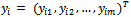
Longitudinal data consist of repeated observations, for the same subject, of an outcome variable. There may be a set of covariates for each subjects. Let 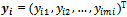be an x 1 vector representing the observed sequence of the outcome variable recorded at time t = 1,2, ... , , for the ith subject, i=1,2, ...., n. Also, assume that x_ij = (x_it1, x_it2, ..., x_itp) is an 1x p vector of p covariates observed at time t. Thus, X_i is an m_i x p matrix of covariates corresponding to the ith subject taking the form:

.

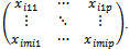For simplicity we can assume that m_i=m.

The primary focus is on the dependence of the outcome on the covariates[3,5]. In other words, we are usually interested in the inference about the regression coefficients, in the usual linear models of the form

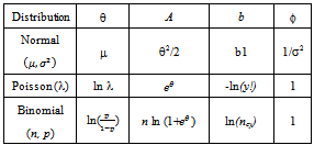
where is a p x1 vector of the regression coefficients. It is usually assumed that the errors, , are independent and identically normally distributed. Therefore, these models are not used in situations when response

variables have distributions other than the normal, or even when they are qualitative rather than quantitative. Examples include binary longitudinal data.

To solve this problem, Reference[18] introduce the generalized linear models (GLM) as a unified framework to model all types of longitudinal data[13, 15, 24]. These models assume that the distribution of Y_it ( i = 1, ..., n, t = 1, 2, ..., m) belongs to the exponential family. The exponential family distributions can be written in the form:

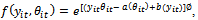(1)

where a(.) and b(.) are specific functions defined according to the underlying distribution of the exponential family. Some examples of univariate distributions are given in Table (1). The parameters and. Also is the scale parameter and it is treated as a nuisance parameter when the main interest is in the regression coefficients[13]. The distribution in Equation (1) is the canonical form and is called the natural parameter of the distribution.

The first two moments of in Equation (1) are given by

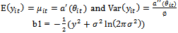(2)

For the GLM, the linear combination of the parameters of interest, , are equal to some function of the expected value of , i. e., where is a monotone and differentiable function called the link function. From Equation (1) and Equation (2), we can write the inverse of the link function as. Note that a link function in which (e.g., h is the identity function) is called the canonical link function. It is sometimes preferred because it often leads to simple interpretable reparametrized models. By looking at θ in Table 1, we can see that the canonical link functions that correspond to the given distributions are the identity (normal distribution), the log (Poisson distribution) and the logit (binomial distribution) functions. Hence, the GLM has three elements:

Table 1. Some common univariate distributions of exponential family

1. The random component which is the response variables that are assumed to share the same distribution from the exponential family,

2. The systematic component which is the explanatory variables that produce the linear predictor, and

3. The link function which is a monotone and differentiable function relating the mean and the linear predictor .

The aim of this paper is to obtain the maximum likelihoodestimates (MLE) of the regression parameters for the logit model relaxing the normality assumption. In this case the estimation process is cumbersome and intractable. Hence, MCMC techniques could be alternative choice. We propose and develop the Monte Carlo EM (MCEM) algorithm, to obtain the maximum likelihood estimates. The proposed method is illustrated using simulated data.

The rest of the paper is organized as follows. In Section 2, we review three distinct approaches to model longitudinal data. Also, we introduce the random effect model. Section 3 discusses several alternatives to maximum likelihood estimation for GLM. The EM algorithm and its variant, namely Monte Carlo EM (MCEM), are described and applied to the random effect model in Section 4. In Section 5, we implement the proposed MCEM algorithm to a simulated binary data. The results obtained from the simulated data are presented in Section 6. Finally, conclusions are given in Section 7.

2. Modeling Longitudinal Data

There are three distinct strategies for modeling longitudinal data. Each strategy provides different way to model the individual in terms of, taking into consideration the possible correlation between the subject’s measurements.

2.1. The Marginal Model

In this approach two models are specified; one for the marginal mean, , and the other for the marginal covariance, In other words, we assume a known structure for the correlation between a subject'smeasurements. The two more natural generalization of the diagonal covariance matrix (case of uncorrelated measurements) are the uniform and the exponential correlation structures. Modelling the mean and the covariance separately has the advantage of making valid inferences about even when an incorrect form of the within-subject correlation structure is assumed.

2.2. The Transition Model

This approach combines the assumptions about the dependence of on and the correlation among repeated into a single equation. The idea behind this approach is that correlation within subject arises because one response is explicitly caused by others. We can specify a regression model for the conditional expectation, , as an explicit function of and the other observations on the same subject. The function is a function of , where is the set of all observations on the subject i except at time t.

For longitudinal data, it is natural to reduce the set to include only observations prior to time t; . A well known example of the transition model is the first-order autoregressive model in which depends on the past history in only through the preceding measurement. Note that the covariance matrix for in this case corresponds to the marginal model with exponential correlation structure.

2.3. The Random Effects Model

This model assumes that the correlation among a subject's measurements arises from sharing unobserved variables. That is, there are random effects which represent unobserved factors that are common to all responses for a given subject. These random effects vary across subjects[8].

Using the GLM framework, we assume that, conditional on the unobserved variables (), we have independent responses from a distribution belongs the exponential family, i.e., has the form in Equation (1) and the conditional moments are given by

.

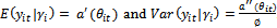The general specifications of the generalized linear mixed model (GLMM) are:

1. The conditional mean, , is modelled by

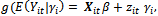where is an appropriate known link function. The and are the outcome variable, the covariates and the regression coefficients vector respectively. The 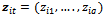is an 1x q subset of associated with random coefficients and is a q x 1 vector of random effects with mean 0 and variance D.

2. The random effects, , are independent realizations from a common distribution.

3. Given the actual coefficients, , for a given subject, the repeated observations for that subject are mutually independent.

Hence, the GLMM is an extension of GLM that includes random effects in the linear predictor, giving an explicit probability model that explains the origin of the correlations [9,10].

Note that for linear model, where the response variable has a normal distribution and the identity link function is used, the random effect model coincides with the marginal model assuming the uniform correlation structure.

3. Estimation of GLM

The method of maximum likelihood is the theoretical basis for parameter estimation in GLM. However, in longitudinal data framework, the presence of within subject correlation renders the use of standard maximum likelihood estimation methods to be problematic. The reason behind this problem is that there are no multivariate generalization to non-normal distributions. As a result, Reference[11] introduce the generalized estimating equations (GEE) method. This method does not make use of the underlying multivariate distribution. It uses certain information associated with the marginal distribution rather than the actual likelihood, which is referred to as quasi-likelihood method[1, 12, 13].

References[11] and[25] introduce a class of estimating equations to account for correlated measurements of longitudinal data. The GEEs can be thought of as an extension of quasi-likelihood to the case where the variance cannot be fully specified in terms of the mean, but rather additional correlation parameters must be estimated. Several alternative methods for analyzing longitudinal data can be implemented using the GEEs, assuming different designs or structures of the correlation matrix[26, 27]. It is difficult to adapt the GEEs for the GLMM. This is due to the fact that the GEEs work most naturally for models specified marginally, not for the GLMMs which are specified conditionally on the random effects[14]. The GEEs, by themselves, do not help to separate out different sources of variation. In addition, they are not direct technology for best prediction of random effects.

The penalized quasi-likelihood (PQL) is another alternative to the maximum likelihood estimation when correlated data are to be incorporated in the GLM. In this approach a penalty function is added to the quasi-likelihood to prevent the random effects from getting too “big”. This method works well for the GLMM when the conditional distribution of the data given the random effects is approximately normal. However, the method can fail badly for distributions that are far from normal[14]. One possible reason for this drawback is the large number ofapproximations needed to solve the integration of the logquasi-likelihood with the additional “penalty” term.

As can be seen, the alternatives to ML fail to work well for many of the GLMMs. Therefore, the classical method remains favourable even though incorporating random factors in the linear predictor of the GLM leads to difficult-to-handle likelihoods. To overcome this difficulty, approaches for approximating or calculating and then maximizing the likelihood are explored.

4. Likelihood Function for GLMM

The GLM often leads to means which are non-linear in parameters, or models with non-normal errors. Also, it leads to missing data or dependence among the responses. This results in a non-quadratic likelihood function in the parameters. Hence, it gives rise to nonlinearity problems in ML estimation[16, 19, 23].

Recall the notation for the GLMM from Section 2.3. Let denote the observed data vector of size m for the ith subject. The conditional distribution of given (the random effect vector for the ith subject) follows a GLM of the form in Equation (1) with linear predictor . The vector 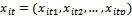represents the tth row of, the model matrix for the fixed effects, . The 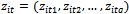represents the tth row of, the model matrix for random effects, , corresponding to the ith subject.

We now formulate the notion of a GLMM:

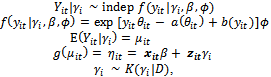(4)

where K(.) is the density function of the random effect with variance-covariance matrix D.

The probability of any response pattern (of size m), conditional on the random effects is equal to the product of the probabilities of the observations on each subject, because they are independent given the common random effects.

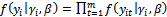Thus the likelihood function for the parameter and D can be written as:

(5)

The above likelihood is analytically intractable except for normal linear models. Traditionally, ML estimation, in these situations, is carried out using numerical iterative methods such as the Newton - Raphson (NR) method and the Fisher scoring method. Under reasonable assumptions of the likelihood and a sufficiently accurate starting value, the sequence of iterations produced by the NR method enjoys local quadratic convergence. This is regarded as a major strength of the NR method, for more details see[17].

However in applications, even fairly simple cases, these methods could be tedious analytically and computationally. The EM algorithm offers an attractive alternative for iterative ML estimation in a variety of settings involving missing data and incomplete information.

4.1. The EM Algorithm

The EM algorithm[2] is a method to obtain the ML estimates, in presence of incomplete data, which avoids an explicit calculation of the observed data log-likelihood. The EM algorithm iterates two steps: the E-step and the M-step. In the E-step, the expected value of the log-likelihood of the complete data, given the observed data and the current parameter estimates, is obtained[22]. Thus the computation in the M-step can be easily applied to pseudo-complete data. The observed (incomplete) data likelihood function always increases or stays constant at each iteration of the EM algorithm. For more details see[17].

A typical assumption in the GLMM is to consider the random effect, , as missing data. The complete data is then and the complete data likelihood is given by

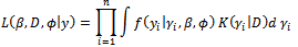Although the observed data likelihood function in Equation (5) is complicated, the complete data likelihood is relatively simple. In other words, the integration over the random effects in Equation (5) is avoided since the value of (the missing data) will be simulated during the EM algorithm and will be no longer unknown.

The log-likelihood is given by

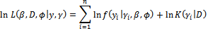(6)

The choice of to be the missing data has two advantages. First, upon knowing, the are independent. Second, in the M-step, where the maximization is with respect to the parameters and D, the parameters and only in the first term of Equation (6). Thus, the M-step with respect to and uses only the GLM portion of the likelihood function. So, it is similar to a standard GLM computation assuming that is known. Maximizing with respect to D, in the second term, is just maximum likelihood using the distribution of after replacing sufficient statistics (in the case that K(.) belongs to the exponential family) with the conditional expected values.

For the GLMM of the form in Equation (4), at the (r + 1) iteration, starting with initial values and, the EM algorithm follows the steps:

1. The E-step (Expectation step)

Calculate the expectations with respect to the conditional distribution using the current parameters' value and

(a)

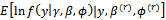(b)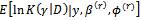

2. The M-step (Maximization step)

Find the values

(a) that maximizes 1 (a).

(b) that maximizes 1 (b).

If convergence is achieved, then the current values are the MLEs, otherwise increment r = r + 1 and repeat the two steps.

4.2. The Monte Carlo EM Algorithm (MCEM)

In general, the expectations in the E-step above, cannot be obtained in a closed form. So we propose using the Monte Carlo Markov Chains (MCMC) techniques[6, 20, 21]. A random draw from the conditional distribution of is obtained. Then the required expectations are evaluated via Monte Carlo approximations.

The Metropolis-Hastings algorithm can be implemented to draw a sample from the conditional distribution of . A candidate value is generated from a proposal distribution Q(.). This potential value is accepted, as opposed to keeping the previous value, by a probability

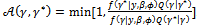(7)

The proposal distribution can be chosen as Q(.) = K(.), the density function of the random effect. This leads to a simplified form of the ratio in the probability of acceptance as

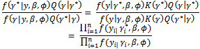This calculation only involves the conditional distribution of

Incorporating the Metropolis algorithm into the EM algorithm, starting from initial values and, at iteration (r + 1),

1. Generate L values from the conditional distribution using the Metropolis algorithm and the current parameters' values and

2. The E-step (Expectation step)

Calculate the expectations as Monte Carlo estimates

(a)

(b)

3. The M-step (Maximization step)

Find the values

(a) that maximizes 2 (a).

(b) that maximizes 2 (b).

If convergence is achieved, then the current values are the MLEs, otherwise increment r = r + 1 and go to step 1.

5. Simulation Study

The proposed method is evaluated using simulated data set. The response variable is assumed to be binary variable.

5.1. Simulation Setup

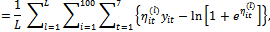
The number of subjects is fixed at 100 subjects and the time points are chosen as 7 occasions. Binary responses are generated, conditionally on the random effect, from a Bernoulli distribution with mean. The random intercept logit model is used.

The parameters values are chosen as . The binary covariate Trti is set to be 1 for half of the subjects and 0 for the other half. The continuous covariate Time is independently generated from normal distribution with mean vector (0 1 2 3 6 9 12) and standard deviation vector (0 0.1 0.2 0.3 0.5 0.6 0.8). Note that, for each subject i, the 1st value of the Time covariate will always be 0. The random intercepts are obtained as such that. Standardized random intercepts are generated from lognormal distribution Ln N(0; 1). The lognormal density is chosen to represent a skewed distribution whose support does not cover the whole real line unlike the normal distribution.

This setup is the same as in[7] to enable us to compare our results with those in[7].

In this case the GLMM in Equation (4) is

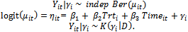(8)

Some remarks are in order about this model. First, = 1 so it drops out from the calculations. Second, we have a single random effect which is common (has the same value) for all the measurements of each subject. Thus are iid from where the variance D is a scalar. Finally, the distribution K(.) will be the lognormal distribution.

5.2. The Logit-Lognormal Model

For this model, the probability density function of the random effect is log-normal with parameters a and b,

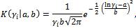where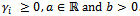

The likelihood function in Equation (5) can be written as:

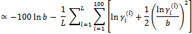
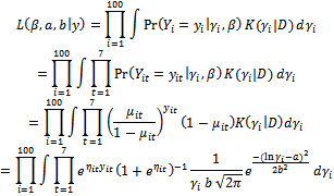Hence, the log-likelihood is given as:

We apply the MCEM algorithm introduced in Section 4.2. Starting from initial values 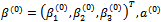and at iteration (r+1), the algorithm proceeds as:

1. For each subject i, generate L values 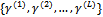from using the Metropolis algorithm with probability of acceptance as in Equation (7) given by

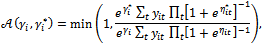where and

2. The E-Step

Calculate the expectations as Monte Carlo estimates

(a)

where

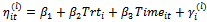(b)

Note that do not show explicitly in this step but they already used in Step 1 to generate the L values of

3. The M-step

Find the values

(a) that maximizes 2 (a).

(b) and that maximizes 2 (b) to use them for the calculation of the standard deviation

If convergence is achieved, then the current values are the MLEs, otherwise increment r = r + 1 and return to step 1.

5.3. Simulation Results

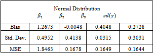
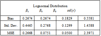
The algorithm described above is implemented using the MATLAB package. Fifty data sets were generated according to the setup in Section 5.1. The random effect was simulated from a lognormal distribution. Then each data set is analysed using the Metropolis EM (MEM) algorithm twice. First, under the normality assumption of the random effects. Second, assuming that the random effects belong to the lognormal distribution. Summaries of the results are given in Tables 2 and 3. Note that Bias, Std. Dev. and MSE are the average bias, standard deviation and mean squared error of the estimates respectively.

Table 2. The Metropolis EM estimates of 50 datasets

Table 3. The Metropolis EM estimates of 50 datasets

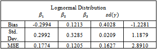
In general, we get better results for the fixed effects when the lognormal density is assumed for the random effect. The parameters' estimates are less variable and the values of the MSE are smaller. The lognormal MEM estimate for is more biased but this is compensated with smaller variance resulting in a lower value of the MSE. On the other hand, the estimate for the standard deviation of the random effect is better for the normal model than the lognormal model.

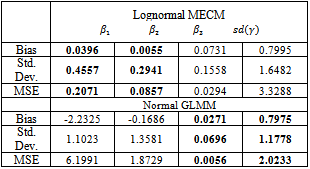
It is clear that there is only a small improvement concerning the estimate of when using the logormal MEM. The bias for is large when using either, normal or lognormal MEM, it is 100% of the true value of the parameter. Therefore, we turn to a modified MEM (MECM) to improve the results. The modification is in the M-step where the parameter vector is divided into two subsets; and (). The maximization of the Monte Carlo expectations calculated in the preceding E-step is replaced by a conditional maximization. In other words, we first calculate that maximize the expectation while is held fixed. Next, we substitute the maximization arguments for and in the expectation function and find the value of that maximizes the function. We repeat this conditional maximization twice. The results obtained for 50 data sets are summarized in Table 4.

Table 4. The lognormal MECM estimates of 50 datasets

Compared to lognormal MEM (Table 3), results are improved when the modified MEM (MECM) is used. We got smaller MSE for all estimates except for and the bias is considerably lower for, and the standard deviation of the random effect. On the other hand, the estimates for, and become more variable.

Table 5. Lognormal MECM and normal GLMM for 100 data sets

We are going to compare our results (the MECM method) with those given in[7]. Table 5 shows the results for the lognormal MECM algorithm of 100 data sets and also the results for the normal GLMM given in[7]. The smaller values, when comparing the two models, are written in bold. A significant improvement can be seen when the lognormal MECM algorithm is used to calculate the estimates for fixed effect and. Results for are good for both lognormal MECM and normal GLMM models, however, the latter gives better values. Finally, MECM algorithm produces more variable estimates for resulting in a higher value for MSE.

6. Conclusions

In this paper, we developed a Monte Carlo EM algorithm to estimate regression parameters for a logit model with lognormal random effects. The proposed method was applied to simulated binary data. A modified M-step was used to improve the results but a trade off between small values for bias and small variability must be made. In general, the obtained results are acceptable when comparing the MEM estimates to those calculated using the normal GLMM.

Further work is to apply the proposed method to larger data sets. We can develop the MEM to logit model with different distribution for the random effect, namely, gamma distribution which is a natural conjugate for the binary data. This work is under investigation now.