-
Paper Information
- Next Paper
- Paper Submission
-
Journal Information
- About This Journal
- Editorial Board
- Current Issue
- Archive
- Author Guidelines
- Contact Us
International Journal of Probability and Statistics
2012; 1(3): 19-35
doi: 10.5923/j.ijps.20120103.01
Statistical Inferences on Uniform Distributions: The Cases of Boundary Values Being Parameters
 Abstract
 Reference
 Full-Text PDF
 Full-Text HTML
Ismail Erdem
Baskent University Faculty of Science and Letters Department of Statistics and Computer Science Baglica, Ankara, 06530, Turkey
Correspondence to: Ismail Erdem , Baskent University Faculty of Science and Letters Department of Statistics and Computer Science Baglica, Ankara, 06530, Turkey.
| Email: |  |
Copyright © 2012 Scientific & Academic Publishing. All Rights Reserved.
If a continuous random variable X is uniformly distributed over the interval and if any of the two boundary values is unknown, it is necessary to make inferences related to the unknown parameter. In this work, for the unknown boundary values of X, some unbiased estimators based on certain order statistics and sample mean are suggested. These estimators are compared in terms their efficiencies. The most efficient unbiased estimator is used to provide confidence intervals and tests of hypotheses procedures for the unknown parameter (the unknown boundary value).
Keywords: Uniform Distribution, Order Statistics, Unbiased Estimators, Efficiency, Confidence Intervals, Tests of Hypotheses
Article Outline
1. Background
- The books and articles, listed in the reference list of this study with the reference numbers from[1] to[18], and many more not in the list, studied order statistics in such a way that every aspects of the topic has already been well explored. However, there is no inferential study, as far as I am aware of, on the boundary values of the uniform distributions. This work aims at the determination of good estimators for the boundary values of uniform distributions. Based on the determined good estimator, construction of confidence intervals and procedures for the test of hypotheses are established. For illustration, a simulation study is conducted and summaries of the simulation study are provided. The raw data and computations are provided in the appendix of this paper.
2. Introduction
- A uniformly distributed continuous random variable, assuming real values in the interval
 , has the following probability density function (pdf)
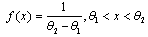 | (1) |
 and
and  will be
  and
and , the smallest and the largest order statistics, respectfully.
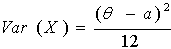
 and
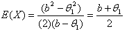
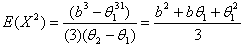
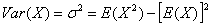
and  need to be estimated for that each moment of the random variable X is , as shown below, a function of these parameters.
 | (2) |
 be a random sample of size n from a uniform distribution over the interval
 , and let
  ith order statistic, i=1, 2,..., n.The pdf of ith order statistic is obtained by the following general formula, as given in almost all mathematical statistics textbooks, like the ones with the reference numbers[1],[2],[3],[4],[6], and[7].
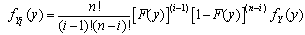 | (3) |
 is the cumulative distribution function (cdf) of the distribution, and
  is the pdf of the random variable ( ith order statistic)
  .Specifically, if the pdf given in (1) is used we obtain the following cdf.
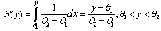 | (4) |
 and
and .
. | (5) |
 | (6) |
 , and
, and . To take advantage of the computational simplicity lets introduce the following transformations.
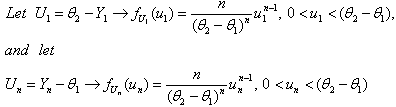 | (7) |
 | (8) |
 | (9) |
 | (10) |
 . It then follows that
 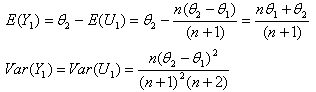 | (11) |
 are exactly the same.Hence,
 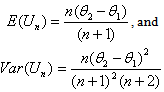 From (7) we get
 . It then follows that
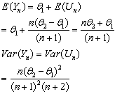 | (12) |
3. Statistical Inferences Related to the Parameter of 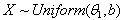 Distribution
3.1. Estimation of the Parameter  of the Distribution
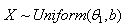 by the First Order Statistic
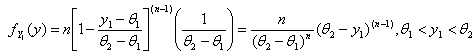
- A uniformly distributed continuous random variable X, over the interval
 , where b is given constant, has the following pdf
 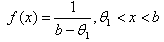 The MLE of
  of
of  will be
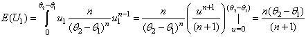
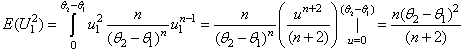
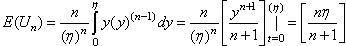
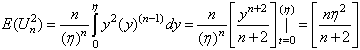
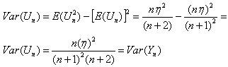
  and its expected value and variance are from Equations given in (11),
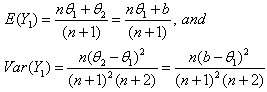 | (3.1.1) |
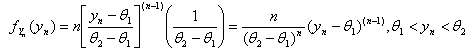
 , based on the first order statistic is
 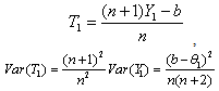 | (3.1.2) |
3.2. Estimation of the Parameter  of the Distribution
 by the Last Order Statistic
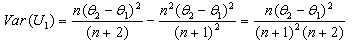
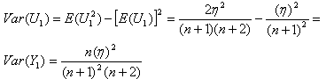
- Another estimator of
 of
of  will be
  and its expected value and variance are from Equations given in (12),
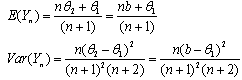 | (3.2.1) |
 as a function of the last order statistic
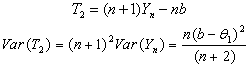 | (3.2.2) |
3.3. Estimation of the Parameter of the Distribution
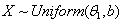 by
by 
- If
 then its pdf is
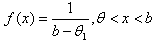 . Then by equation (1), as given below:
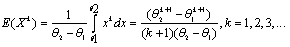 For k=1 and
 | (3.3.1) |
 ,
, | (3.3.2) |
 we obtain
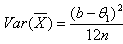
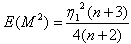
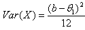 . For any distribution, if the sample mean is
  , for any random sample of size n, the followings hold true.
 , and
, and 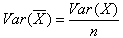 Hence, for
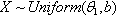 ,
, 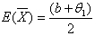 | (3.3.3) |
 | (3.3.4) |
 will be
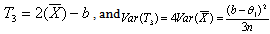 | (3.3.5) |
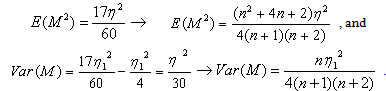
3.4. Estimation of the Parameter  of the Distribution
 by the Sample Median M
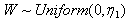
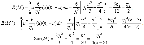
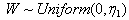
- If
 then
then  is uniformly distributed over the interval
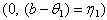 To take advantage of computational simplicity, the parameter
  (and in turn
  of X), of the distribution
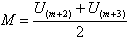
 , is to be estimated by the sample median.Sample Median (M):Let
  is a random sample of size n from
  The sample median M, depending on if n is odd or even, is obtained as follows.If
  are ordered, in the order of their magnitude, we obtain the following order statistics.
  .
. If n is odd:
  If n is even:
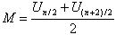
3.4.1. Estimation of the Parameter θ1 of the Distribution X∼Uniform(θ1, b) by the Sample Median n is Odd
- Theorem 3.4.1. If
 and if an odd sized random sample is taken from this distribution then for the sample median M,
 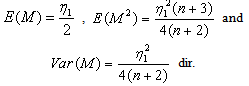 Proof: Proof will be given by induction.for n=1:
 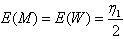 and
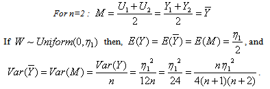
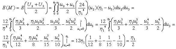
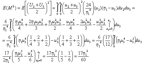
and 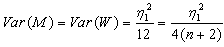 .For n=3: the sample median is
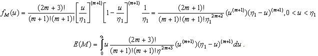
  .The pdf of
  is to be obtained, by the use of (3), as follows.Since,
 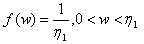 and
and 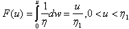 , then
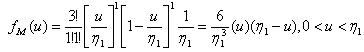 | (3.4.1) |
 Similarly, for n=5,
  and from (3)
 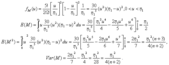 For n=2m+1, then
  .
.  Now, let’s assume that the following hold true for any n=2m+1.
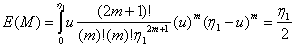 | (3.4.2) |
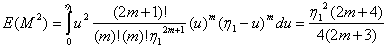 | (3.4.3) |
 .
. If we let
  then in accordance with (3.4.2) and (3.4.3) we conclude the following.
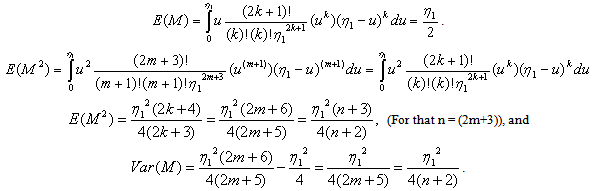 For the case of n being an odd number, the proof is completed.
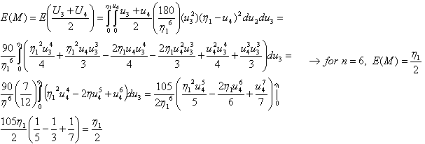
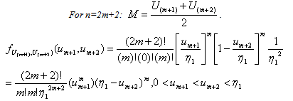
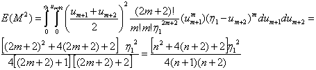
3.4.2. Estimation of the Parameter θ of the Distribution X∼Uniform(θ1, b) by the Sample Median n is even
- Theorem 3.4.2 If
 and if an even sized random sample is taken from this distribution then for the sample median M,
 Proof:Note: If n is even, then the sample median is
 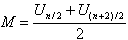 . To compute the expected value and the variance of M we need to have the joint pdf of
  . For any random sample taken from the distribution of
 , joint pdf of the ordered statistics
 , and
, and , (r < t) can be obtained by the use of the following general formulation as given in[6].
  | (3.4.4) |
 For n=4:
  . The joint pdf of
 and
and  is obtained as given below.Since,
  and
and 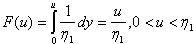 according to (3.4.5) the joint pdf is
  | (3.4.5) |
 For n=6:
  , the joint pdf of
  and
and  is obtained as given below.:
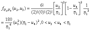 | (3.4.6) |
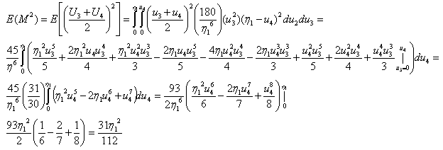
 Now, let’s assume that the following, given in (3.4.7) and (3.48), hold true.
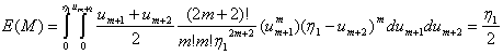 | (3.4.7) |
 | (3.4.8) |
 The joint pdf of
 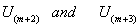 is obtained as follows.
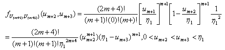
 | (3.4.9) |
 , observing the identity between (3.4.7) and (3.4.10) we conclude the following.
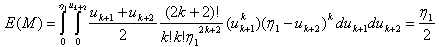 | (3.4.10) |
 | (3.4.11) |
 , observing the identity between (3.4.8) and (3.4.12) we conclude the following.
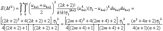 | (3.4.12) |
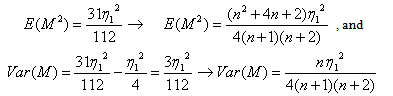
3.4.3. Unbiased Estimators of θ1 for X∼Uniform(θ1, b) by M
- n is odd:
 ,
,  , and
, and 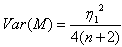 Where
Where  , hence an unbiased estimator of
  as function of is M
 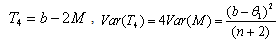 | (3.4.13) |
 ,
,  , and
, and 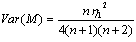 .
.
|
 for the Distribution
  and their variances
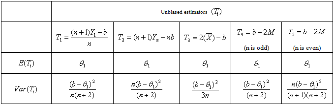
 , hence an unbiased estimator of
  as function of is M
  ,
, | (3.4.14) |
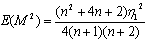
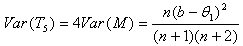
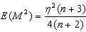
 We see that, for n >1, the most efficient unbiased estimator, among the ones as given above, is
 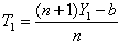 .
.4. Confidence Interval for the Parameter  of the Distribution
- The most efficient unbiased estimator of
 is seen to be
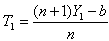 . By the use of the pdf of
  we can construct a
  confidence interval for
 . As it is shown before
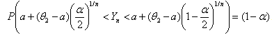
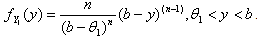 .By the use of following probability statement we can obtain a confidence interval for
 .
.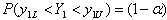 | (4.1) |
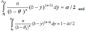 If we let
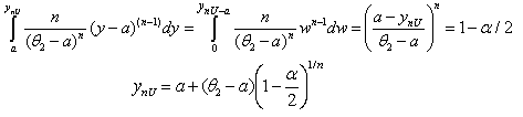
  then the following are true:
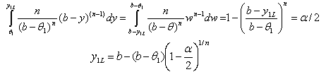 | (4.2) |
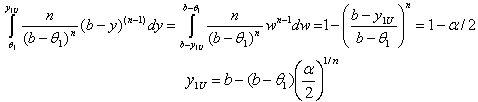 | (4.3) |
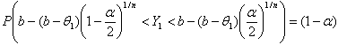 Solving the above inequalities for
 we obtain the following Confidence Interval.
 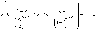 | (4.4) |
 confidence interval for
  :
: 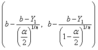 | (4.5) |
5. Tests of Hypotheses Related to the Parameter  of the Distribution
|
 for the Distribution
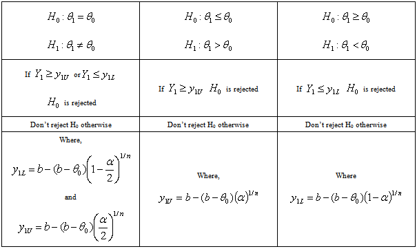
 is to be tested against to any proper alternative hypothesis, a plausible test statistic is to be
  for that the most efficient unbiased estimator is
 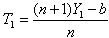 , which is a linear function of
  .If the level of significance is chosen to be, then the decision rules, as given in the following table, are applicable. It is concluded that the best unbiased estimator, among the ones suggested, of the parameter for the uniform distribution over
  is
is .Since T1 is a linear function of the first order statistic Y1, construction of confidence interval and tests of hypotheses procedures are related to and dependent upon the observed value of the first order statistic Y1 and the chosen level of significance
  .
.6. Statistical Inferences Related to the Parameter of  Distribution
6.1. Estimation of the Parameter θ2 of the Distribution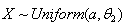 by the First Order Statistic
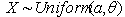
- A uniformly distributed continuous random variable X, over the interval
 , has the following pdf.
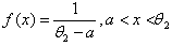 If
If  then,
then, 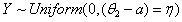 and its pdf is as given below.
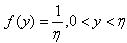 .If a random sample of size is taken from the distribution of Y, then the ordered statistics will be denoted by
  .The parameter of this distribution,
  , can be estimated by
  . The pdf of
  is given below.
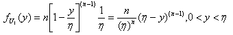 | (6.1.1) |
 | (6.1.2) |
 then the following will hold true.
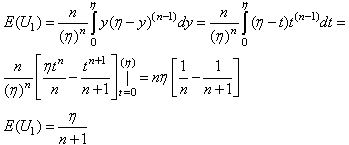 | (6.1.3) |
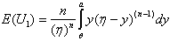
 of
of 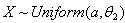 will be
  and its expected value, from the transformation
 , is obtained as given below.
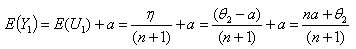 | (6.1.4) |
 | (6.1.5) |
 and
and  .
. | (6.1.6) |
 , then
 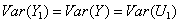 .
. | (6.1.7) |
 as a function of
 .
. | (6.1.8) |
6.2. Estimation of the Parameter  of the Distribution
 by the Last Order Statistic
- If we want to estimate the parameter
 of
of  by
by ,
, | (6.2.1) |
 | (6.2.2) |
 | (6.2.3) |
 is
is .Since,
  , then the following will be true.
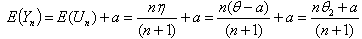 | (6.2.4) |
 | (6.2.5) |
 | (6.2.6) |
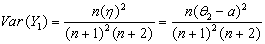
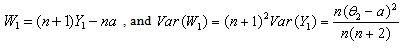
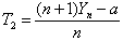
 .From (6.2.4) we obtain an unbiased estimator for
  as a function of
 .
. | (6.2.7) |
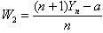
6.3. Estimation of the Parameter  of the Distribution
 by the Sample Mean
- If
 then the pdf is
 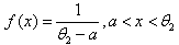 , and
, and 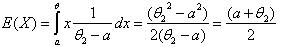 ,
, 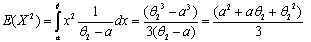 ,
,  . For any distribution, if the sample mean is
  , for any random sample of size n, the following hold true.
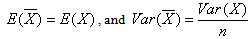
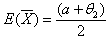 | (6.3.1) |
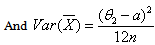 | (6.3.2) |
 , as function of the sample mean
  .
.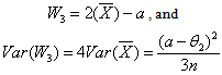 | (6.3.3) |
6.4. Estimation of the Parameter  of the Distribution
 by the Median M
- A uniformly distributed continuous random variable X , over the interval
 , has the following pdf
 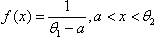 If
If  , then as it is stated in Note 1,
 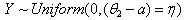 and its pdf is as given below.
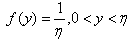 .Estimation procedures and the findings, related to the parameter of
 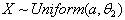 , will be exactly the same as the one given in sections 1.4.1 and 1.4.2, with the exception that
  In other words, the statements of Theorem 1.4.1 and Theorem 1.4.2 hold true. That is: if n is odd then,
  ,
,  , and
, and 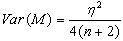 ,If n is even, then
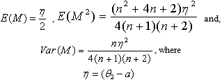 The unbiased estimators of as functions of the sample median M are as follows:
 (when n is odd),
  (when n is even).The variances of these unbiased estimators are:
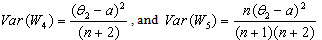
6.5. Comparisons of Unbiased Estimators in Terms of Their Efficiencies
- The unbiased estimators and their comparisons are given in Table 3. We see that, for n >1, the most efficient unbiased estimator among the ones given above, is
 .
.7. Confidence Interval for the Parameter  of the Distribution
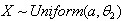
- The most efficient unbiased estimator of is seen to be
 . By the use of the pdf of
  we can construct a
  confidence interval for. As it is shown before
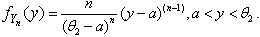 .By the use of following probability statement we can obtain a confidence interval for
 .
.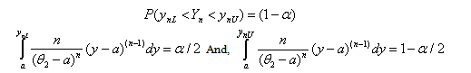 | (7.1) |
 then the following are true:
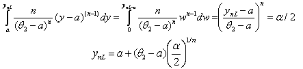 | (7.2) |
 | (7.3) |
|
 for the Distribution
  and their variances
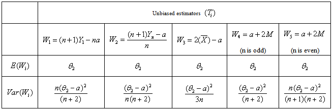
|
 of
of 
 .Solving the above inequalities for
  , the following Confidence Interval is obtained.
 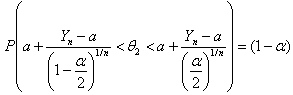 | (7.4) |
- A
 confidence interval for
  is given as follows.
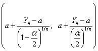 | (7.5) |
8. Tests of Hypotheses Related to the Parameter  of the Distribution
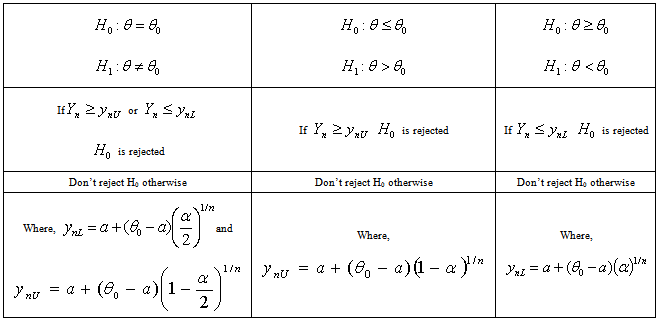
- If
 is to be tested against to any proper alternative hypothesis, a plausible test statistic is to be
  for that the most efficient unbiased estimator is
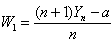 , which is a linear function of
 .If the level of significance is chosen to be
 , then the decision rules, as given in the following table, are applicable.
 9. Conclusions
- For uniform distributions, of the types
 , and
, and  , some unbiased estimators for the unknown boundary values
  and
and  are suggested. Among the suggest estimators, the most efficient estimator is selected. By the use the most efficient estimators, confidence interval and tests of hypotheses procedures are established.
 10. Simulation Study
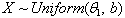
- To see the match between the established theoretical findings and the empirical results, a simulation study on a uniform distribution over the interval
 is carried out. 100 independent samples of size 100 are drawn from this uniform distribution. From each sample the first order statistic
 , the last order statistic
 , sample mean
 , sample medians
  (for n=100), and
  for n=99) are computed. Unbiased estimator values are computed from each sample. Summary of the simulation results are given in the following Table 5.
|
 , summary statistics,
  of 100 observations are obtained. Values of five different estimators for
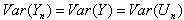
 , namely T1, T2, T3, T4, and T5 are computed from each sample by the use of proper summary statistics. The second and third columns of Table 5 contain the computed means and the variances of each summary statistics and of estimate values for
 . From Table 5, we observe that T1, T2, T3, and T5 are unbiased estimators of
 . Among these unbiased estimators T1 is the best (the most efficient) estimator, for that it has the smallest variance.In the same line, values of five different estimators for
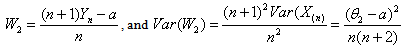
 , namely W1, W2, W3, W4, and W5 are computed from each sample by the use of proper summary statistics. From the second and the third columns of Table 5, we observe that W1, W2, W3, W4 and W5 are unbiased estimators of
 . Among these unbiased estimators W2 is the best estimator, for that it has the smallest variance.By using the formula (2.5), a 95% confidence interval is computed for
  from each sample. Exactly 95 out of 100 confidence intervals contained the parameter value 5 of
  .Similar procedures are followed for
 . By the use of the formula (5.5), 95% confidence intervals for
  are computed. 94 out of 100 confidence intervals contained the parameter value 10 of
 .Simulation study results are seen to be in accordance with the theoretical findings.