Hoa Tran
Department of Computer Information Sciences, Fordham University, NY 10458, Bronx
Correspondence to: Hoa Tran , Department of Computer Information Sciences, Fordham University, NY 10458, Bronx.
| Email: |  |
Copyright © 2012 Scientific & Academic Publishing. All Rights Reserved.
Abstract
As the tool to predict the collapse in terms of finance of a company, the probability of ruin plays a crucial role. The interest rate, initial compounding assets, together with ruin time, ruin function will be discussed for the new directions of observing the chance of being collapsed of the company. As the interest rate becomes larger, the observation is the probability of ruin will be smaller. Random walk, Brownian motion and the connection with Capital Asset Pricing Model also will be addressed. The models can assist decision makers or investors to make decision to choose between insurance and investment risk.
Keywords:
Probability of Ruin, Time of Ruin, Ruin Function, Interest Rate, Random Walk, Brownian Motion
1. Introduction
Since Dassios[5], Harrison[7] and Paulsen[15], several models for Risk Analysis had been established, but there are no connections to the CAPM, Sharpe[16]. As was pointed out by Dassios[5], these processes should provide a standard theory for studying applications in insurance risk theory. The Poisson arrival condition will be relaxed to a general renewal arrival process, Karatzas[10]. The service payment model will follow the replacement model in Gihman[6]. The analysis of integral representation will be given by Moriconi[14], the properties of which were subsequently investigated by Lintner[11]. In this paper, relevant facts that affect the probability of ruin so that people can determine the stability of companies. The models for the corruption of an event can be viewed as the stage of Stochastic Risk, using the parameters to determine its stability.
2. Stochastic Risk Model
Let 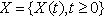 be a stochastic process with stationary, independent increments, finite variance, and
  . We call this as income process. Given a positive y of initial assets and a positive interest rate 𝛽, we define
 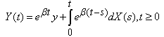 | (2.1) |
the asset process Y by Let  be a Poisson process with arrival rate λ , and let W1,W2 be independent and identically distributed random variables with distribution F. Let c be a finite constant, take
 Let
Let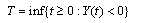 Call T the time of ruin and r(.) the probability of ruin, then
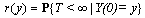 | (2.2) |
Assume that the process X is defined on a probability space and has stationary, independent increments with E[X(t)] = μt and Var[X(t)]=  , where
  and
and  .Let
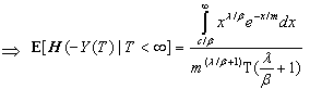
.Let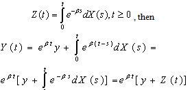 Theorem:We have
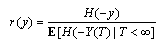 | (2.3) |
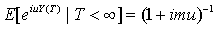
where H is the distribution function of Z(∞).
3. Ruin Problems versus Interest Rate
As the interest rate β increases, the ruin function r(.) will get smaller. This fact can say a lot about the way of controlling the collapse in finance of the company. The chance of being collapsed in finance will be smaller if the interest rate is raised or higher.For the characteristic function of X(t) we have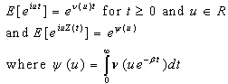 From[6]. the representation can be
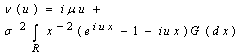 | (3.1) |
where G is a probability distribution in R.Suppose that  The exponential function is
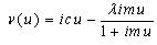 then
then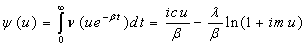 | (3.2) |
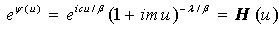 Invert H then
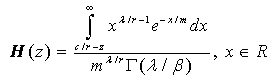 | (3.3) |
 The probability of ruin is
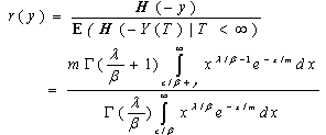 | (3.4) |
4. Connections with CAPM – Risk Model
Let Rl = Investment return of security iRm= Return on market portfolio mRf= Return on risk-freeThe security market line is a relationship between expected return and risk for all individual securities and portfolio in the market.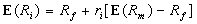 where r is a risk sensitivity determined by
5. Numerical Results
Assume that 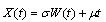 where W is a standard Wiener process, then
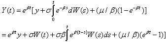 | (5.1) |
Thus we can obtain a representation of the present value process as a rescaling of Brownian motion, | (5.2) |
Combining (5.1) and (5.2), we have the asset process as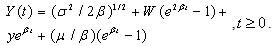 From (5.2) we conclude that Z () has the Gaussian distribution
 where a =
 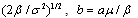 and
and  is the standardized normal distribution function. We finally have
Table 5.1. Values of probability of ruin r(y) as σR increases
 |
| |
|
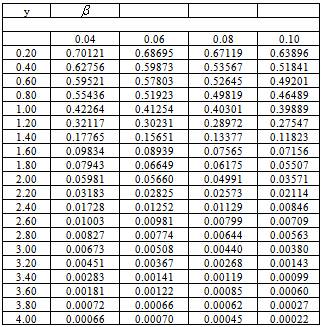
Table 5.1 gives r(y) when β= 0.10, σR= 0.00, 0.10, 0.20 and 0.30, p =1, σR = 1 and y = 0.20, 0.40, 4.00. We see that the impact of a stochastic interest rate is fairly small when the probability of ruin is large, but becomes increasingly important as the probability of ruin decreases. For large value of y we see that the uncertainty in return on investments may increase the probability of eventual ruin several times.Table 5.2. Values of probability of ruin r(y) as interest rate increases
 |
| |
|
Table 5.2 gives r(y) when β = 0.04, 0.06, 0.08 and 0.10, σR = 1, p =1, σP = 1 and y = 0.20, 0.40, 4.00. The set of those data confirm the validity of conjecture 4.3.1, as for the control of risk, raising the interest is one of the ways. The data show that the impact of interest rate setting is fairly big when y is small enough, then the sensitivity of interest rate could be a matter to for the safe investments.
6. Conclusions
The number of problems in Stochastic Risk Theory and its applications had been shown; in particular, the probability of ruin had been examined carefully with many properties. The relationship of ruin function and the interest rate creates vast applications in finance and insurance industry, where the investors can use it to model their business model as well as helping their investing decisions for many business op portunities.The compound Brownian motions and the limit theorems were used to manifest the convergence of ruin probability, which could even strengthen the underlying theory of stochastic risk; the compound asset processes and its associating risk will be determined by Brownian approximation.
References
| [1] | M. Avellaneda, A. Levy and A. Paras, “Pricing and Hedging Derivative Securities in markets with Uncertain Volatilities,” Appl. Math. Finance 2 (1995), 73-88 |
| [2] | M. Avellaneda and A. Paras, “Dynamical Hedging Strategies for Derivatives Securities in the Presence for Large Transaction Costs,” Appl. Math. Finance 1, (1994), 165-193 |
| [3] | P. Bickel and K. Doksum, Mathematical Statistics, vol. 1, 2nd edition. Prentice Hall, New Jersey, 2001 |
| [4] | P. Billingsley, Probability and Measure, 3rd edition. Wiley, New York 1995 |
| [5] | A. Dassios and P. Embrechts, “Martingales and Insurance Risk,” Comm. Statist. – Stochastic Model 5 (1989) 181-217 |
| [6] | I. Gihman and A. Skorohod, Introduction to the Theory of Random Processes. Saunder, Philadelphia, PA, 1969 |
| [7] | J. M. Harrison, “Ruin Problems with Compounding Assets,” Stochastic Process. Appl. 5 (1977) 67-79 |
| [8] | J. Hull, Options, Futures and Other Derivatives, 5th edition. Prentice Hall, New Jersey, 2003 |
| [9] | N. L. Jacobs and H. R. Petit, Investments. Irwin, Homewood, IL, 1984 |
| [10] | I. Karatzas and S. E. Shreve, Brownian Motions and Stochastic Calculus. Springer, New York, 1988 |
| [11] | J. Lintner, “The Valuation of Risk Assets and the Selection of Risky Investments in Stock Portfolios and Capital Budgets,” Review of Economics and Statistics 47, no. 1, (February 1965) 13-37 |
| [12] | H. McKean, Stochastic Integrals. Academic Press, 1969 |
| [13] | R. Merton, “Option Pricing when the underlying stock returns and are discontinous,” J. Financ. Econom. (1976), 125-144 |
| [14] | F. Moriconi, “The submartingale assumption in risk theory,” Insur. Math. Econom. 5 (1986) 295-304 |
| [15] | J. Paulsen, “Risk Theory in a stochastic economic environment,” Stochastic Process. Appl. 46 (1993), 327-363 |
| [16] | W. Sharpe, “Capital Asset Prices: A Theory of Market Equilibrum under Conditions of Risk,” Journal of Finance 19, no. 3 (September 1964), 425-442 |
 Abstract
 Reference
 Full-Text PDF
 Full-Text HTML