1. Introduction

During a period of heavy rainfall, satellite and terrestrial microwave communications that operate at frequencies higher than 10 GHz which may have signal interruptions [1]. Thus, point-to-point (PP) connectivity may impede continuous content streaming [2]. Link errors must be fully eliminated, especially during live broadcasting [3]. The signal along wireless communication networks is weakened by rain, a natural occurrence [4,5]; hence, mitigating rain attenuation is required to maintain a constant stream of content. Based on this assumption, dynamic fade mitigation strategies may be used in conjunction with fade prediction models that can predict the link's condition. In light of this, steps may be taken to guarantee that the link will remain completely operational for communication services even during a storm. Many researchers have employed an artificial neural network (ANN) for rainfall forecasting and demonstrated that the ANN may provide acceptable results after training [1,6–9]. In this study, rain attenuation is predicted and classified using the adaptive neural fuzzy inference system (ANFIS), a neural network employing a feedforward multilayer perceptron neural network (MLPNN) trained with Levenberg-Marquardt algorithm (LMA) for dynamic rain attenuation mitigation.

This research aims to comparatively analyze adaptive techniques for good quality of service on terrestrial and satellite network systems in Nigeria, especially during intense storms. The objectives are to deduce attenuation using 5-year rain rate data from a tropical location in Akure Nigeria (using the synthetic storm technique and ITU-R attenuation model); formulate an adaptive technique to predict and control signal to noise using hybrid adaptive measures (fuzzy logic and an artificial neural network), and further compare a proposed adaptive mitigation measure to improve Quality of Service (QoS) during intense weather conditions.

The techniques presented in this research can be adapted to create a stable and effective algorithm that can effectively manage signal propagation for network service providers as well as manage the quality of signals in channels impacted by attenuation due to weather at high frequencies. It can also serve as a noticeable contribution to improving the signals transmitted via satellite networks and invariably aid in improving satellite services. Many studies have been carried out by researchers to improve the quality of service on wireless and satellite networks. Crane and co-workers carried out a researched the prediction of the effect of rain on satellite communication in temperate regions [10]. His research shows that the effect can be estimated if the distribution of rain intensity is known in both time and space. Harb and colleagues investigated the quality of service improvement in weather-impacted satellites using the Markov model to predict weather attenuation that can maintain quality of service via an intelligent awareness control system [11–14]. Nomura and co-researchers proposed a learning method of fuzzy inference in which the inference rules express the input-output relation of the data and are obtained automatically from the data gathered by specialists [15]. In this method, triangular membership functions were tuned through experience. The learning speed and generalization capabilities of this method were higher than those of a conventional back propagation neural network. Dhafer and co-workers also investigated how to simplify the factors for an ad-hoc network on mobile phones using fuzzy techniques, and it was deduced that higher throughput does not usually mean a high quality of service [8]. Furthermore, the system developer expressed the knowledge acquired from the input-output data in the form of fuzzy inference rules. Eyob and colleagues worked on enhanced adaptive code modulation (ACM) for rainfall fade mitigation in Ethiopia, and the results show that a neuro-fuzzy inference system can be employed to enhance mitigation techniques while maintaining link availability [9]. This study aimed to adopt a hybrid-adaptive mitigation measure to maintain the quality of signals along the terrestrial and satellite propagation links in a tropical location. The list of abbreviations and their respective meaning are listed in Table 1.

Table 1. List of abbreviations and meaning

The remaining sections of the paper are as follows. Section 2 gives the background knowledge of the work and methodology adopted. The adaptive modelling schemes and model predictors are presented in Section 3. The implementation and simulation strategies are demonstrated in Section 4. Section 5 presents a detailed results and discussions. Section 6 concludes the paper with discussions on future directions.

2. Background Knowledge

2.1. Modelling Based on Machine Learning Using Experimental Data

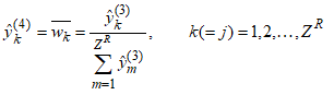
The goal of machine learning (ML), a division of artificial intelligence (AI), is to create systems that can learn from the data they consume and enhance their performance. Artificial intelligence is a general term that describes robots or systems that can imitate human intellect. Every learning strategy is data-driven. The system is trained using data sets. These data sets are gathered and applied to training. In this study, the system received 2732 rows of data based on rain rate measurement based on vertically-looking micro rain radar as presented in Figure 1. To validate the data used, tipping bucket rain gauge measurements from archived data of the Communication Research Group, Physics Department, Federal University of Technology, Akure have been used. It comprises of five years of rain data of one minute integration time series from 2013–2018.

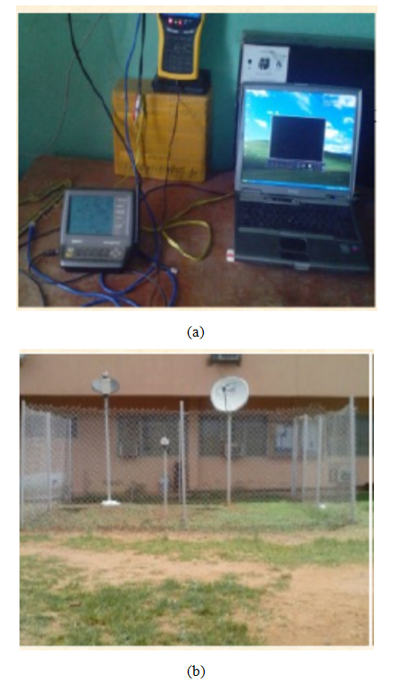Figure 1. Setup of the micro rain radar: (a) Observatory centre and (b) micro rain radar station

The cumulative distribution function and, later, the diurnal influence on the signal were determined by analyzing the time series rain rates. At both the Super High Frequency (SHF) and Extremely High Frequency (EHF) bands, rain-induced attenuations (RA) were deduced using the SST model. The model utilized in this study is human-derived and based on human observations and experiences. It is known as mechanisms for supporting decision-making in networks as discussed in the next sub-section. The typical perception of models is that they are human-derived and serve as a foundation for machine learning. Some machine learning techniques, however, create their models free of any human-derived structure.

To achieve this practically, a system that maps an input to an output needs to be trained. The neural network and fuzzy logic are two examples of such systems [16,17]. Systems for machine learning must be taught through training [18]. Learning Systems frequently employ models, which offer mathematics in order to learn a mapping. The learning machine's structure (models or data) must be modified once the system receives an input and its associated output. This has some similarities to regression or curve fitting. When additional inputs are added, the system ought to be able to provide the right results if we have enough training pairs. Problems can occur if there are not enough training sets, if the training data is not diverse enough, or if it fails to encompass the entire range.

Unsupervised learning and supervised learning are the two types of machine learning [19]. Specific training sets of data are applied to the system during supervised learning. Although the "training sets" were created by people, the learning is supervised. However, this does not necessarily imply that humans are actively verifying the outcomes. Labelling is the process of categorizing the system's outputs for a certain set of inputs. In other words, you clearly state which outputs or results are correct for every set of inputs. The generation of training sets might take some time. However, tremendous efforts must be made to guarantee that the training sets will provide acceptable training results; in order to ensure that the system will produce the right results when real-world data are presented. The whole range of anticipated inputs and planned outputs must be covered by them. Test sets are used to validate the findings after the training.

2.2. Time-Series Using Synthetic Storm Techniques

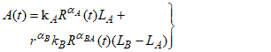
Synthetic Storm Techniques (SST) are physical-mathematical radio propagation method that can be used to generate reliable rain attenuation time series by converting a rain rate time series at a specified site into a rain attenuation time series. Local parameters such as rain rate, length of the signal path through the rain cell, and rain cell velocity at the site under investigation are required in the SST [20]. Moreover, by applying the SST method, rain attenuation time series at any frequency and polarisation can be generated for any slant path above approximately 10 degrees, as long as the hypothesis of isotropy of the rainfall spatial field holds in the long term. The SST method is very useful for designing communication satellite systems and improving their performance for calculating rain attenuation over a satellite path. The troposphere's vertical structure divides into two levels when it rains. A is regarded as the rain layer, and B is the melting layer. The expression is given as

(1)

where A(t) denotes the time series generated attenuation, R^αA(t) gives the time-series rain rate at rain layer A, R^αB(t) is the time-series rain rate at melting layer B, L_A and L_B gives the slant paths at layer A and B, respectively. α_A, and k_A are the constant that are estimated for layer A (for the temperature of precipitation is 20°C as reported in the ITU-R Recommendation P.838-3 [21,22] and α_B, and k_B denotes the constant that are estimated for layer B (where the temperature of the precipitation is 0°C) [23].

2.3. Block Diagram Description of the Proposed Machine Learning Scheme for Good QoS

The proposed system makes use of different weather conditions (such as rain) occurring at various times are taken into account, supported by accurate background data, to enhance the effectiveness of our decision system. The block diagram of the proposed machine learning scheme uses random weather event, regular query and knowledge base in conjunction with ANFIS decision algorithms, core computing intelligent model and data prediction scheme based on neural network to determine good quality of service (QoS) as illustrated in Figure 2. This system utilizes the Levenberg-Marquardt algorithm within an Adaptive Neuro-Fuzzy Inference System (ANFIS) using neural network to perform predictions and decision-makings in ensuring consistent good quality of service (QoS).

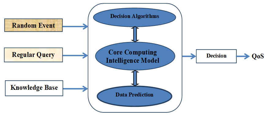Figure 2. Block diagram of the proposed machine learning scheme for supporting decision-making in networks

The adopted system uses various random weather conditions, such as rain, which are queried for necessary precision at different times and supported by accurate background knowledge to enhance the effectiveness of good decision-making process.

3. Adaptive Modelling Schemes and Model Predictors

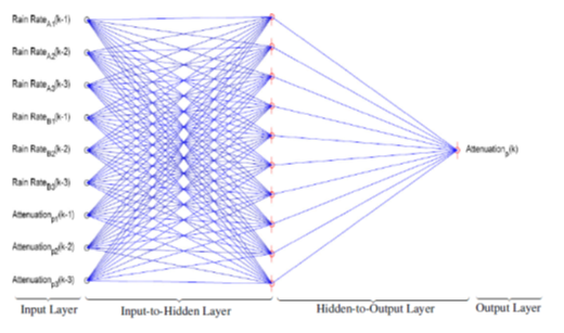
3.1. The Feedforward Multilayer Perceptron Neural Network (MLPNN)

The neural prediction scheme used in this paper is based on the series-parallel architecture shown in Figure 3 where the system is in parallel with the NN identification model (in the dashed box) and tapped delay line (TDL) denotes tapped delay line memory used to store temporal NN input information. It consists of a training algorithm and the NN model. Assuming that the input-output data pair of the system taken over NT period of time is available [19]:

(2)

where N is the number of data pair and T the sampling interval. Assuming also that the input-output data pair in (7) is available, and m and n are known. The inputs to the NN, via an -TDL and -TDL, are the past m-inputs and n-outputs contained in which is obtained from defined in (2); where and .

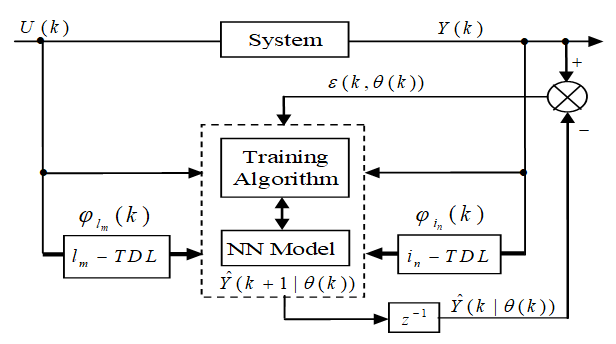Figure 3. Series-parallel structure for neural network model identification

The NN considered of Figure 3 has a dynamic recurrent architecture as shown in Figure 4, since it contains temporary memories elements (TDL) and feedback, in this case, from the output of the system rather than the output of the NN model. Note that series-parallel structure shown in Figure 3 correspond to the autoregressive with exogenuous input (NNARX) model predictor. This is the so-called teacher forcing method where the network output is forced to follow the system outputs which leads to faster online training in real-time. With this method, the actual NN model, shown in Fig. 4, can be trained as a FNN.

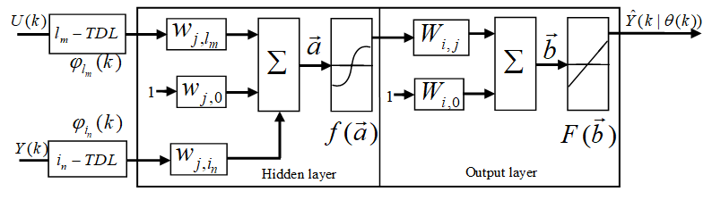Figure 4. Multilayer perceptron neural network (MLPNN) model architecture

The internal architecture for the proposed for the NN model is a MLP NN with two-layers (one hidden and one output layer) shown in Fig. 4. Decomposing in (14) into the input and output parts as 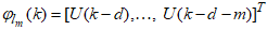and 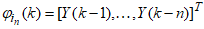respectively, the output of the NN of Figure 3 can be expressed in terms of the network parameters of Figure 4 as

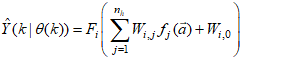(3)

where

and j is the number of hidden neurons; and and are the hidden and output weights respectively; and are the hidden and output biases; is a linear activation function for the output layer and is an hyperbolic tangent activation function for the hidden layer defined here as:

(4)

Bias is interpreted as a weight acting on the input clamped to 1. Here, we use the term “joint weight” to imply both the network weights and biases that constitute .

The neural network output prediction problem then translates to a nonlinear minimization where the error estimates

(5)

between the outputs of the true system output and the predictor output in (3) is minimized in some sense and used to adjust and update recursively to obtain an optimal parameter vector . The minimization of (5) to obtain can be expressed as:

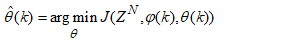(6)

where is formulated as a mean square error (MSE) type cost function given as:

(7)

Several techniques for solving (5) exist in literature and different methods for adjusting and updating have also been reported [19,24–26].

The training algorithm used here is the Levenberg-Marquardt algorithm (LMA) from the Deep learning Toolbox of the MATLAB [24]. The network training method is as follows. At time k, given , , a small initial as well as the available and ; the training algorithm then computes the a priori output estimate . At time is available which is used to compute the a posteriori output estimate and the error (5) is used to adjust until is obtained or certain stopping criteria is satisfied. Note that in (5) is now given by (3) and we still seek the value of in (6).

3.2. The Adaptive Neuro-Fuzzy Inference System (ANFIS)

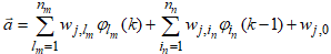
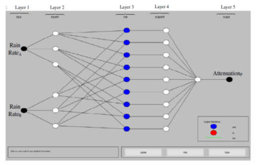
The adaptive neuro-fuzzy inference system (ANFIS) was introduced to create a method for intelligent systems design whose behaviour or pattern inherent in a given dataset is unknown which could be obtained using neural network techniques from where fuzzy rule-based intelligence can be automatically generated and incorporated using the fuzzy inference system (engine). A typical architecture of a five-layer ANFIS is shown in Figure 5. The commonly and most widely used five-layer shown in Figure 5 ANFIS architecture including the one implemented in MATLAB® and Simulink® [24] which has been adopted for used in this study. For completeness, consistency and simplicity, each of these five layers is described below with their accompanying mathematical descriptions [27].

Figure 5. The architecture of the five-layer ANFIS

Layer No.1 - Inputs Normalization Layer (Complement Coding)

The nodes of this layer simply transmit the input signals to the next layer. The ANFIS uses the technique of complement coding to normalize the input training data. Complement coding is a normalization process that replaces an n-dimensional input vector with its 2n-dimensional complement coded form u' such that:

(8)

where . Complement coding helps avoiding the problem of category proliferation when using fuzzy-ART for data clustering. Having this in mind, we can write the I/O function of the first layer as follows:

(9)

where Z^N is the number of input variables.

Layer No.2 - Fuzzy-AND Operation

These nodes represent a fuzzy set and they calculate the degree of activation of each membership function. Each node is characterized by the parameters of the fuzzy set it represents. Each node in this layer performs a fuzzy-AND operation. Similar to the other ANFIS networks, the T-norm operator of the algebraic product is selected. These results make each node’s output to be the product of all its inputs:

(10)

where Z^T is the number of output variables.

The output of each node in this layer represents the firing strength (or activation value) of the corresponding fuzzy rule. Note that the number of the fuzzy rules equals the number of input term nodes. The latter is common for all the input variables. Therefore, each fuzzy rule may be assigned an index kequal to the corresponding index j of the input term node, which is common for each input linguistic variable.

Layer No.3 - Normalization of Each Rule Firing Strength (Fuzzy Rules Strength Normalization Layer)

The nodes in this layer calculate the firing of the rule, usually through the product operator. The output of the k-th node in this layer is the firing strength of each rule divided by the total sum of the activation values of all the fuzzy rules. This results in the normalization of the activation values of all fuzzy rules:

(11)

where Z^R is the number of fuzzy-based rules.

Layer No. 4 – Rule Consequent Layer

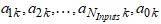The nodes of this layer correspond to the consequent of the rule. Each rule node in layer 3 has an equivalent node in this layer. The latter calculates the algebraic function of the Takagi-Sugeno Khan (TSK) rule. Both constant and linear function types are allowed. Each node k in this layer is accompanied by a set of adjustable parameters and implements the linear function:

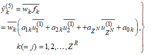(12)

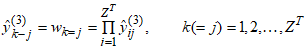
The weight is the normalized activation value of the k-th rule calculated with the aid of (12). Those parameters are called the consequent parameters or linear parameters of the ANFIS system and are regulated by the training algorithm.

Layer No.5 - Output Layer

The single node of this layer produces the output of the network, performing the weighted average defuzzification process. For the proposed HANFA-ART system, this layer consists of one and only node that creates the network’s output as the algebraic sum of the node’s inputs:

(13)

Equations (8) through (13) shows how the input vector is fed through the network layer by layer to the predicted, estimated or classified output for a particular given problem.

4. Implementation and Simulation Strategies

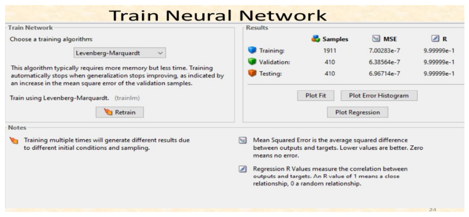
The five-year rain rate data was evaluated using feedforward multilayer perceptron neural network (MLPNN) trained with the Levenberg-Marquardt algorithm (LMA). Adaptive neuro-Fuzzy inference system (ANFIS), and neural network. As shown in Figure 3 is the neural architecture; the neural set-up comprises the two inputs (rain rate at layer A and rain rate at layer B) and output (Attenuation or quality of service (QoS)).

In this study, both the feedforward multilayer perceptron neural network (MLPNN) predictor of Figure 3 and the Adaptive neuro-fuzzy inference system (ANFIS) of Figure 5 were trained using the Levenberg-Marquardt algorithm (LMA). The 2,731 data was split into 70% (1,911) training data for both MLPNN and the ANFIS; 15% (410) was used for validation while 15% (410) was reserved for the trained network testing [17,19,25,26]. If the output prediction (QoS) are poor, the procedure is repeated by adjusting the hidden layer neuron for MLPNN, joint weight (network weights and biases) and the number of iteration for performance improvements while maintaining the same number of three past values for performance comparison until satisfactory performance was achieved.

The system is trained using the training data sets and validated using the validation data sets. These data sets are gathered and applied to training. In this instance, the system received 2732 new pieces of data. The rain rate and attenuation time series for frequency 12.25 GHz are shown in Figure 6. The relations show a trend whereby, as the rain rate increases, attenuation also rises. For example, at a rainstorm's 180.6 mm/hr over 1100 seconds time interval, attenuation was 50 dB, which had a significant impact on the propagating signal, while at a drizzle's rain rate categorization of 30.4 mm/hr, the attenuation was 5.4 dB.

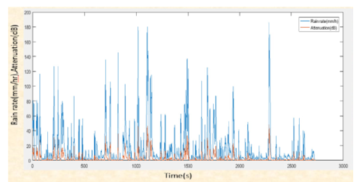Figure 6. Time Series Rain Rate Data and Attenuation at 12.25GHz

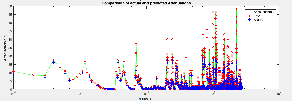
5. Results and Discussion

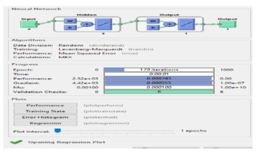
The MLPNN and the ANFIS were trained using the LMA through simulation studies and the structure of the simulated MLPNN and the ANFIS networks are shown in Figure 7 and Figure 8 respectively. The LMA modifies the weight and bias parameters in accordance with LMA optimization scheme. In Figures 9 and 10, the Levenberg-Marquardt optimization procedure determines the update of the parameters using the adaptation parameter (Mu). Figure 6 displays the gradient and Mu-values of the trained network. Mu is the control parameter for the neural network training technique; its initial value was 0.001, and its maximum value is 1e10.

Figure 7. Structure of the simulated feedforward multilayer perceptron neural network (MLPNN)

Figure 8. Structure of the simulated ANFIS network

Figure 9. The graphical user interface (GUI) for the MLPNN training

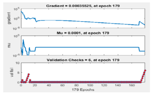Figure 10. Convergence parameters for MLPNN training after 179 iterations

The dotted-line attribute is the best-trained epoch as shown in Figure 11 which designates the iteration at which the validation performance was at its lowest. Before coming to an end, there were another six (6) repetitions of training. It is probable that some over-fitting occurred if the test curve grew considerably before the validation curve did. The creation of a regression plot, which depicts the relationship between the network's outputs and the targets (Figure 12), is the next stage in verifying or validating the network. The network outputs and targets would be precisely equal if the training was flawless, but in reality, this is rarely the case. For instance, using commands, we might make a regression plot. The first command figures out how the trained network will react to each input in the data set. The targets and outputs from the training, validation, and test subsets are extracted by the other instructions or commands. Three regression graphs are produced by the last command for training, testing, and validation. As shown in Figure 8, the three graphs reflect the training, validation, and testing data. Each plot's dashed line illustrates the perfect outcomes, which are outputs equal to targets. The solid line displays the best-fitting linear regression line between the outputs and the targets. The link between the outputs and the targets is shown by the R value. If R = 1, then the connection between the outputs and the targets is exactly linear. There is no linear relationship between outputs and targets if R is close to zero [24,28]. Figure 13 shows the result of the trained data for the two layers and the attenuation. The regression results are all close to one.

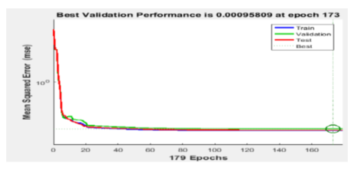Figure 11. Convergence results for training, validation, testing based on mean squares error (MSE)

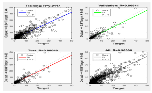Figure 12. Linear regression ® fitting result for the MLPNN training

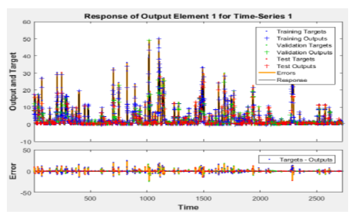Figure 13. The MLPNN QoS output predictions and the prediction errors

With a very low mean square error (MSE) of 7e-7 for the train at 1911 samples and a regression rate close to 0.999 e-1, the trained MLPNN output time series is shown in Figure 14. The MSE of 6.386e-7 at 410 samples for validation and a 410 test sample MSE of 6.967e-7 are obtained from Figure 14, which clearly illustrates the value for the train, validation, and test.

Figure 14. Performance metrics of the trained neural network

The design of the adaptive neural fuzzy inference system with inputs (rain rate at layers A and B), outputs (attenuation), and corresponding membership functions are shown in Figure 15. The input parameters are the Rain rate at layers A and B, and the output value is Attenuation. Low, average, and high values are assessed for the input parameters.

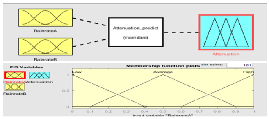Figure 15. Inputs, rule editor, output and membership function editor of the ANFIS network

A comparable prediction model was created in a similar way to verify the research's central idea. With the same input and output data, we employed an Adaptive Neural Fuzzy Inference System (ANFIS). A neural network and a fuzzy inference system (FIS) are combined to create the Neuro-Fuzzy system. It has the advantages of both soft computing technologies together. By creating an if-then rule, it inherits the neural learning technique used to modify the membership function parameters from the neural network and the structure from FIS (Figure 16) [8,10]; nonetheless, sample data must be trained, tested, and checked to confirm the outcome. The trained FIS is confirmed with testing data that is different from the training data we used to train it, with 70% of the data—the 1910 sample data—used for training and the remaining 30% for testing the trained FIS network. Figure 17 demonstrates that there is a perfect match at the 1000 epoch, and Figure 18 shows that the training result has an error of 0.024287.

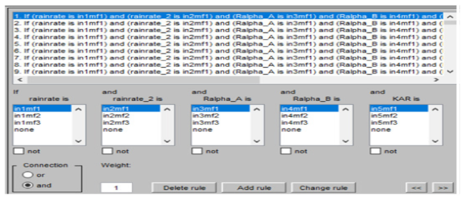Figure 16. Automatically generated fuzzy rules by the trained ANFIS

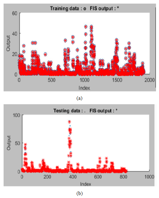Figure 17. The ANFIS output predictions: (a) training data and (b) test data

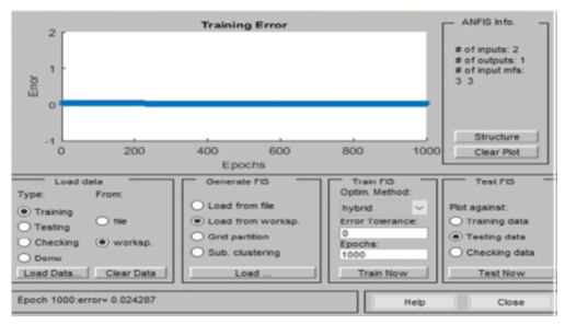Figure 18. Training errors for the ANFIS network at 1000 iterations

Performance Comparison of the Machine Learning Models

The number of iterations (or epochs) for both models—the neural network and the adaptive neural fuzzy inference system—was fixed at 1000. The neural model's best match was discovered after 179 iterations with a mean square error rate of 7e-7, whereas the ANFIS was 0.024287 after 1000 iterations. A table comparing the two models and their relative predicted outcomes based on error rates is shown in Table 2. The MLPNN model and ANFIS predictions for attenuation are compared to the actual attenuation in Table 2. For example, the predicted values for the multilayer perceptron neural network (MLPNN) and Adaptive Neural Fuzzy Inference System (ANFIS) are 10.79 dB and 9.31 dB, respectively, at actual attenuation of 10.76dB. Similarly, the MLPNN and the ANFIS predict values of 8.55 dB and 7.27 dB with an actual attenuation value of 8.56dB.

Table 2. Predicted and actual values of attenuation

Figure 19 presents a plot comparison of the rain rate, attenuation, and predicted values during a time span of 500 seconds. For the values at the 500-second time period, there was a cluster. However, the predicted values also increased in tandem with the rising rain rate and attenuation values. According to MLPNN and ANFIS, the attenuation, for instance, is 48 dB at a rain rate of 180 mm/hr, while the predicted values are 46.88 dB and 35.92 dB, respectively. Similar to Figure 20, Figure 21compares the actual and predicted attenuation. At 10-second intervals, both the actual and predicted attenuations have a fair fix and good matches. The comparison of the logarithms in Figure 21 demonstrates the cluster and matches, especially at intervals of 1000 seconds. Back propagation neural network and adaptive neural fuzzy inference system projected appropriate values, as indicated in all attenuations for specified values. The two models actually predicted accurate values as corroborated in Figure 21.

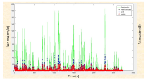Figure 19. Comparison of actual rain rate, attenuation, and predicted attenuation

Figure 20. Comparison of actual rain rate, attenuation, and predicted attenuation

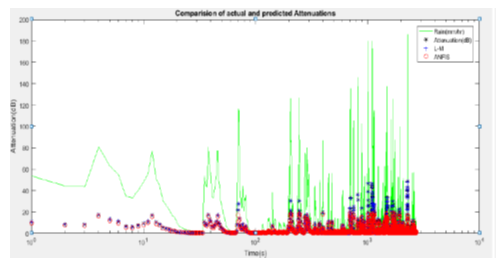
Figure 21. Logarithmic comparison of actual and predicted attenuation

6. Conclusions and Future Direction

6.1. Conclusions

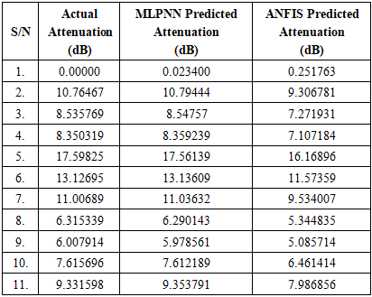
Five-year rainfall data has been utilized in this study to assess various prediction methods and suggest mitigating strategies to enhance service quality and control signal to noise. Comparing the ANFIS and our actual output attenuation revealed an overall percentage difference of 0.2517%, whereas the Levenberg-Marquardt neural network and our actual output attenuation revealed a difference of 0.0234%. This suggests that, despite the fact that both MLPNN and ANFIS are beneficial for prediction purposes, attenuation prediction in neural networks is more accurate and suitable. This is corroborated in the results for both MLPNN and ANFIS, which exhibit the same pattern- and graphic-based trend. It was then deduced that the MLPNN result shows a more accurate and reliable prediction with lesser error and thus is a good decision support system for mitigating rain attenuation. With the predicted values, our model can accurately manage the loss of signal (attenuation) and provide necessary mitigation techniques for an effective signal to maintain quality of service, especially under intense weather conditions.

6.2. Future Direction

Future research should expand the scope of this study by incorporating longer-term and more diverse meteorological datasets to improve the robustness of attenuation prediction models. Extending rainfall data beyond five years, and integrating additional climatic variables such as temperature, humidity, cloud density, and wind speed, could further enhance model generalization under varying environmental conditions.

Furthermore, hybrid deep-learning architectures such as deep convolutional neural networks (Deep CNN), long short-term memory (LSTM) networks, random forest, support vector machine (SVM), and deep neuro-fuzzy systems should be investigated to determine their potential to outperform conventional MLPNN and ANFIS models in highly random weather scenarios. Future studies may also examine real-time adaptive learning techniques, enabling models to update continuously as new rainfall and attenuation data become available, thus improving accuracy during dangerous weather conditions.

Another promising direction is the development of intelligent, automated mitigation frameworks that combine predictive outputs with proactive countermeasures. These may include dynamic power control, adaptive modulation and coding, site diversity, and antenna beam optimization, triggered autonomously based on predicted attenuation levels. Implementing such systems within real communication networks will allow for end-to-end performance assessment and validation.

Finally, integrating satellite-based rainfall measurement data, IoT-enabled weather sensors, and GIS-based spatial analysis can support the creation of more broad attenuation maps. These tools will provide network designers and operators with better insights for infrastructure design, resilience planning, and long-term service quality improvement.