Yousef M. Alshehri, Joseph Chung
Department of Computer Science and Software Engineering, Monmouth University, West Long Branch, NJ, United States
Correspondence to: Yousef M. Alshehri, Department of Computer Science and Software Engineering, Monmouth University, West Long Branch, NJ, United States.
| Email: |  |
Copyright © 2019 The Author(s). Published by Scientific & Academic Publishing.
This work is licensed under the Creative Commons Attribution International License (CC BY).
http://creativecommons.org/licenses/by/4.0/

Abstract
Wireless Mesh Networks (WMNs) could feasibly be used as an organization’s secondary backup network due to their properties such as dynamic self-organization, self-configuration, self-healing, decentralized management, and inexpensive implementation. This backup network could help allow an organization's business to continue in case of an extended main network outage. This paper involved the study and implementation of WMNs to evaluate the feasibility of a WMN as a backup network. A variety of devices were used in this research including Raspberry Pi 3 devices, network switches, and Wi-Fi adapters. The key devices were the Raspberry Pi’s which were used as mesh routers (MRs). Three Local Area Network (LAN) topographies were provided via the MRs using external Wi-Fi adapters. We tested the three topologies using an extension of the Optimized Link State Routing Protocol (OLSR). We measured three network performance parameters from the MRs and LAN clients to Mesh Router 3 (MR3), a gateway node. The measured parameters were throughput, delay/jitter, and a proportion of lost datagrams out of total datagrams sent. The parameter results were analyzed to evaluate the performance of the mesh networks. Several factors that may affect the measured parameters are discussed such as physical obstacles, wireless interference, inter-node distance, and multiple hops.
Keywords:
Wireless Mesh Networks, Optimized Link State Routing Protocol, Network Performance
Cite this paper: Yousef M. Alshehri, Joseph Chung, Evaluation of Wireless Mesh Network Implementation for Backup Network Access, International Journal of Networks and Communications, Vol. 9 No. 3, 2019, pp. 103-114. doi: 10.5923/j.ijnc.20190903.03.
1. Introduction
What happens if the main network of your organization goes down? How would the organization’s users access local networks and/or the Internet to keep the organization functioning? One of the solutions could be to have a secondary backup network in place using wireless technologies. An intriguing choice for a backup wireless network is a mesh network. The way that wireless mesh networks work and the cost of building them are two reasons why we have chosen to study the feasibility of a backup mesh network. The properties of mesh networks are the following: dynamic self-organization, self-configuration, self-healing, minimal wiring requirements, and decentralized management. Due to these properties, building a mesh network should be relatively cheap and not time-consuming. Also, maintenance should be relatively easy, and network services provided by a mesh network should be reliable and efficient [1].A mesh network consists of nodes. The nodes in a mesh are of two types: mesh clients and mesh routers. The mesh router nodes are the backbone of the network, and the mesh clients and conventional clients get access to the network through them. Every mesh router node acts as both a host and a router [1]. In this paper, we have built a pilot-scale mesh network using Raspberry Pi devices, personal computers, and commodity hardware. The networks have been configured with various topologies to measure throughput and other performance measures to ascertain whether mesh networking could serve as a secondary organizational network for backup and emergency use.
2. Background
2.1. The Wireless Mesh Networks Overview
A wireless mesh network is considered a special type of ad hoc network due to some similarities between the two networks. A mesh network is a multi-hop wireless network that uses a mesh topology where some nodes are fixed [2]. The properties of mesh networks are the following: dynamic self-organization, self-configuration, self-healing, and decentralized management [1]. Besides these properties, the connection between the mesh network and its clients does not require any routing features or specific software modules to be used by the clients. Due to these properties, mesh networks have been proposed and implemented in places where network access is scarce, such as in third world nations, through projects such as the One Laptop Per Child initiative [3].A wireless mesh network is characterized as a decentralized network due to its mesh topology. These networks consist of two types of nodes. The first type of node is a wireless mesh router and the second is a wireless mesh client [1]. The mesh router node works as an access point for other nodes and is considered part of the self-organized backbone of the network. The mesh clients and conventional network clients get access to the network through the router nodes. Thus, all the traffic to and from mesh clients are relayed by the mesh routers. Wireless client nodes can be any device that has a wireless network interface card. These nodes can connect directly to mesh routers. Meanwhile, devices that are not equipped with wireless, e.g., desktop PCs, can connect to the mesh routers indirectly, through conventional LAN switches that are connected to the mesh routers.In mesh networks, nodes can still communicate with each other even if some nodes no longer work. Because of its self-organization and self-configuration properties, the reliability of mesh networks can be high. When more nodes are added to the network, the reliability tends to increase [4].Due to their properties, wireless mesh networks could be suitable for application in many fields, for example, in home networks to overcome dead zones, in military applications to manage emergencies such as disasters, in communities to provide broadband connectivity within a city or neighborhood, and in organizations such as universities and corporations to provide services such as VoIP [1].
2.2. Architecture of Wireless Mesh Networks
The possible architectures of a wireless mesh network are the following:a. Infrastructure/backbone: This is the most common architecture of WMNs that are built upon different wireless radio technologies such as IEEE 802.11 [1]. Interconnected wireless mesh routers (WMR) form a mesh of self-configuration and self-healing, which is the backbone of the network for conventional clients. Via bridge functionality in some WMRs, wireless networks can integrate and interconnect with the wireless mesh network. Network clients can connect to the network through wireless access points using different radio technologies, directly through WMRs using the same radio technology, or via Ethernet.b. Client architecture: In this architecture, mesh client nodes provide peer-to-peer mesh networking among mesh client devices [1]. Mesh clients perform routing and self-configuration and provide end-user applications to users. No WMRs are needed in this architecture. Usually, one radio technology is used on participating devices.c. Hybrid architecture: Predicted to be the most common mesh architecture in the future, this architecture is simply a merger of the two types of architectures: infrastructure/backbone and client [1]. There are two ways for a mesh client to access the network: the first way is through wireless mesh routers and the second way is via other mesh clients. The infrastructure/backbone sub-architecture provides integrity and interconnection with other networks, while in the client sub-architecture, enhanced connectivity and coverage within the mesh are provided by mesh clients.
2.3. Routing in Wireless Mesh Networks
Routing is based on some metric that is used by protocols to select optimal routing paths. Examples of routing metrics for WMNs are hop count and round trip time [5]. Scalability, reliability, flexibility, throughput, load balancing, congestion control, and efficiency are the requirements that have to be met by routing metrics to ensure good routing performance [6]. Routing protocols in wireless mesh networks can be broken down into the following types:
2.3.1. Proactive Routing
The goal of proactive routing protocols is to maintain up-to-date routing tables of each node in the network topology, where each node has a routing table that represents the whole network topology [7]. Proactive routing protocols keep the network refreshed by sending broadcast route update messages after a constant period of time. Thus, tables are derived for each node in the network. This consumes the bandwidth of the network, while the discovery delay is reduced [7]. Thus, it is suitable for small networks. Some examples of proactive routing protocols are the following: Destination Sequenced Distance Vector Routing (DSDV) and Optimized Link State Routing Protocol (OLSR).
2.3.2. Reactive Routing
Reactive routing is also called on-demand [6]. The routes are calculated by flooding the network with route requests [7]. Thus, new routes are obtained using route requests and route replies. Ad Hoc On-Demand Vector (AODV) is an example of a reactive routing protocol.
2.3.3. Hybrid Routing
The combination of proactive and reactive routing protocols derives another type of routing protocol called hybrid routing. Proactive routing protocols are used when the routing is from a source node to another node in an area within the range of the source node, while reactive routing protocols are used for nodes not in the same zone as the source node. An example of a hybrid routing protocol is the Hybrid Wireless Mesh Protocol (HWMP) [7].
3. Related Works
When implementing a wireless mesh network, design decisions need to be made such as the kinds of devices that will form the network and the routing protocols that will be used to try to optimize performance. These design decisions will also require a study of the stable or transient network clients that are expected to use the network. Regardless of how good the mesh network implementation may look, performance testing and analysis of the test results will be needed to feedback into the design phase. This performance evaluation is a key part of the work described in this paper, in which we evaluate whether a mesh network can perform adequately as a backup network.Babu, Cortés-Peña, Shah, and Krishnan presented an implementation of a wireless mesh network where they implemented and evaluated a five node network, which consisted of four mesh routers and one mesh client, using laptops in an infrastructure-based architecture. They studied and implemented the OLSR and BATMAN routing algorithms and also a modified static routing algorithm [8]. Yuliandoko, Sukaridhoto, Rasyid, and Funabiki implemented a mesh network consisting of 3 mesh routers in a campus building using laptops. They used the BATMAN-ADV routing algorithm along with the delay-tolerant IBR-DTN protocol. They tested and compared four test scenarios in which the locations of the nodes were fixed and then mobile. Finally, they found that the overall performance of the TCP wireless mesh network improved, in terms of throughput, when IBR-DTN was applied [9]. Bhushan, A. Saroliya and V. Singh, using the simulation tool NS-2, simulated a wireless mesh network consisting of 30 mesh routers and 16 mesh clients using two wireless ad-hoc network routing protocols which were AODV and DSR, wherein the scenarios were generated based on specific parameters. Next, they measured performance metrics such as throughput and average delay to evaluate ADOV and DSR. They found that the performance of both ADOV and DSR algorithms were about the same for a static network but found that DSR yields better performance in cases of increasing mobility (varying distance of nodes) in the random waypoint mobility model for mesh clients [10]. Roofnet is one of the earliest and most well-known research projects in the area of wireless mesh networks. Aguayo, Bicket, Biswas, De Couto, and Morris designed and developed a mesh network with the help of volunteers in Cambridge, Massachusetts. The mesh consisted of 50 nodes, where each node was connected to an omni-directional antenna installed on the roof of a building. In Roofnet, they used SrcRR as the routing protocol, which is adapted from the DSR routing protocol; SrcRR basically finds the highest throughput route among multiple routes. Communication between nodes was through multi-hop 802.11b with a maximum of 4 hops. Some nodes--the gateway nodes--were connected to the Internet through wires. They claimed that the throughput was up to hundreds of kilobytes per second [11].In our paper, we have built wireless mesh networks using Raspberry Pi’s and other commonly-available devices with the OLSR routing protocol to test the network’s performance with consideration for the effects of interference and obstacles. Our network consisted of 10 nodes, including mesh clients. We tested three different topologies that included line-of-sight and non-line-of-sight node connections. Our nodes communicated via multi-hop 802.11g using either the Raspberry Pi 3’s built-in Broadcom BCM43438 Wi-Fi adapter or external USB Wi-Fi adapters which were Atheros AR9271-based. The measured throughput reached 32 Mbps in one of the cases.
4. System Components and Implementation
4.1. System Components
There is a variety of hardware that can be used to form mesh networks. For our purposes, we wanted to use hardware that was low cost, easy to set up and take down, portable and low in energy consumption. We decided to build our network using the following equipment:1) Raspberry Pi 3 Model B: The primary devices used in our mesh network. Each Raspberry Pi acted as a mesh router. We used 7 Raspberry Pi’s running the Raspbian OS via the Pi’s SD card slot.2) External Wi-Fi adapters: Five TP-Link TL-WN722N (revision 1) USB Wi-Fi adapters, based on the Linux-supported Atheros AR9271 chipset. We used these adapters to form wireless local networks, to add gateway (Internet provider) functionality to one of the Raspberry Pi mesh routers, and to add Wi-Fi access to client desktop PCs.3) Network switch: A fast Ethernet switch was linked to one of our mesh routers to add wired PCs to the mesh as clients.4) PCs: Desktop computers were used as mesh clients.5) Laptops: Two laptops were used to monitor the network and perform testing.
4.2. Configuration
We configured each Raspberry Pi to be a mesh router. The mesh routers formed the backbone of the mesh network. In addition, some of the mesh routers were also configured as wireless access points, one mesh router was configured as an Ethernet local network router, and one mesh router was also configured as a network gateway to provide Internet access.On each Raspberry Pi, we installed the following required packages from the official Raspbian package repository:• wireless-tools: Needed for setting up and monitoring wireless interfaces.• olsrd: Optimized link-state routing protocol daemon.
4.2.1. Configuration of Mesh Router Nodes
We modified the wireless network interface of each Raspberry Pi to make it a wireless mesh router node via changes to the standard /etc/network/interfaces configuration file. Key configuration options included the wireless interface name (wlan0), private network we would use (10.0.0.0), a static IP address, the wireless channel, wireless ESSID, and wireless ad-hoc mode. When using ad-hoc mode, the Raspberry Pi 3’s built-in Broadcom-based Wi-Fi adapter is limited to 802.11g.
4.2.2. Configuration of Wireless Access Points
To allow two mesh routers to act as wireless access points we added an external USB Wi-Fi adapter (TP-Link TL-WN722N) as the second wireless network interface on those mesh routers. These access point mesh routers were called MR1 and MR5. The resulting additional wireless interface (wlan1) on MR1 and MR5 was configured for access point functionality using the hostapd package [12]. MR1 and MR5 were also configured as DHCP servers.Additional configuration options were added to the /etc/network/interfaces file on MR1 and MR5 to set up the wireless network for clients (192.168.2.0) and the default Internet gateway (MR3 with IP address 10.0.0.3). NAT routing via iptables was also configured on MR1 and MR5.
4.2.3. Configuration of Ethernet Local Network Router
A mesh router (MR4) was set up as an Ethernet local network router using the Raspberry Pi’s default Ethernet interface (eth0). The setup was similar to the wireless access points, including a local network for wired clients (192.168.3.0), default Internet gateway (MR3), DHCP server setup, and NAT routing.
4.2.4. Configuration of Network Gateway
To provide Internet access via our mesh network, we added one of the TP-link TL-WN722N external USB Wi-Fi adapters to one of the mesh routers (MR3) as wireless interface wlan1. MR3 was configured as a gateway node within the mesh. The source of the Internet connection in our tests was a smartphone 4G/LTE connection which would be accessed by MR3 via Wi-Fi tethering. We configured the added wireless interface (wlan1) through the standard /etc/network/interfaces file. Lastly, we configured NAT routing via iptables between wlan0 (wireless mesh) and the Internet (wlan1).
4.3. Implemented Topologies
We studied, planned, and implemented several of mesh network topologies in this research. In planning the topologies, we wanted to ensure that the topologies included the key factors that influence wireless mesh network performance. In this subsection, we present three topologies that were tested using our chosen routing protocol, OLSR.• Optimized Link State Routing Protocol (OLSR):The OLSR protocol is a proactive routing protocol, an optimization of a Link State algorithm [13]. OLSR relies on multipoint relays (MPR). The broadcast packets are only forwarded by some chosen nodes which are MPRs. As a result, packet overhead is reduced because not every node is broadcasting the packets [14]. Since the number of broadcasting nodes is reduced, throughput is increased because the packet overhead is reduced during the process of flooding. In OLSR, MPRs are chosen in such a way that each node communicates with an MPR that is within one hop, where an MPR of a node is its neighbor that has the highest connectivity to other nodes. Paths are advertised between a particular MPR and its MPR selectors. MPRs receive network information from each other. This process eventually creates a complete routing table for each MPR. In classic OLSR, the best path is determined based on the minimum number of hops.The particular implementation of OLSR that we used is the UniK-OLSR implementation hosted at olsr.org [15]. UniK-OLSR extends OLSR by using Expected Transmission Count (ETX, the number of transmissions expected for a packet to be sent to its destination) to select multi-point relays (MPR) to determine the best path, instead of relying on a minimum number of hops [8]. For example, the path with the smallest total ETXs from one mesh router to another router will be chosen, even though the number of hops along this path may be greater than for all other available paths to reach the other router.- OLSRD Daemon Configuration:OLSR is implemented using a daemon (olsrd) on each mesh router through the configuration file, /etc/olsrd.conf. After finalizing the configuration parameters of OLSR [17-19], we configured each mesh router in our topologies as needed.
4.3.1. First Topology, Apartment
As shown in Figure 1, we set up four Raspberry Pi mesh routers (MR1 - MR4) to form the backbone of the network. The mesh routers were located in each corner of an apartment. Mesh router MR1 had a local wireless network associated with its external wireless interface wlan1, while MR4 had a local Ethernet network associated with its Ethernet interface eth0. MR3 (gateway) provided Internet connectivity to the mesh network via a smartphone Wi-Fi tethered hotspot. The dotted green lines indicate all of the available routes in the network. 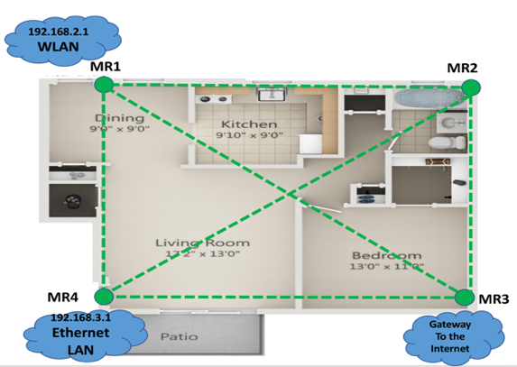 | Figure 1. First topology consisting of four mesh routers |
OLSR-generated routes: In Figure 2, we show the routing paths that were generated after applying the OLSR routing protocol on each mesh router to update the routing tables. The purple dotted lines are the generated routes from each mesh router to MR3 which were 1-hop routes. Network clients that connected to the wireless LAN and Ethernet LAN would be 2 hops away from MR3. The route distances from MR1, MR2, and MR4 to MR3 were 10.8 meters, 8 meters, and 7.3 meters, respectively.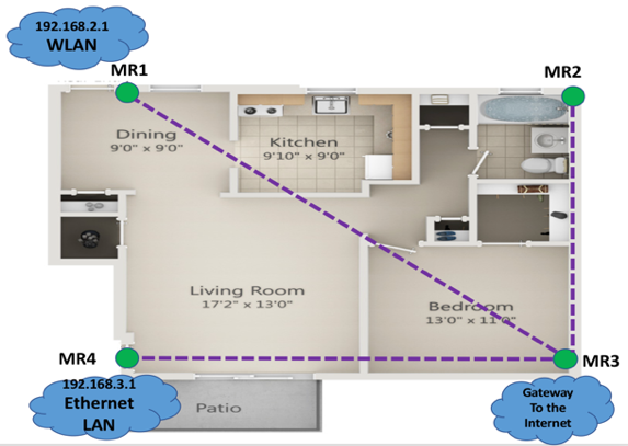 | Figure 2. OLSR-generated routes of the first topology from each mesh router to MR3 |
4.3.2. Second Topology, University Building I
This topology was implemented in an academic building at Monmouth University. As shown in Figure 3, there were seven mesh routers (MR1 - MR7) used to form the mesh backbone. All of the mesh routers were located on the second floor, except for MR5, which was located on the third floor. MR1 and MR5 were configured as Wireless LAN access points using external wireless interface wlan1, while MR4 had an Ethernet LAN associated with its Ethernet interface eth0. MR3 provided Internet access to the mesh via smartphone tethered Wi-Fi hotspot. The green dotted lines show all of the available routes in the mesh.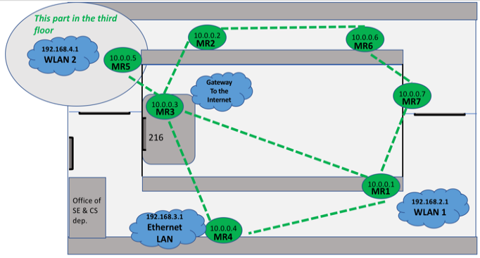 | Figure 3. Second topology consisting of seven mesh routers |
OLSR-generated routes: In Figure 4 below, we show the routing paths generated after applying OLSR. The purple dotted lines show the routes from each mesh router to MR3. Mesh routers MR1, MR2, MR4, and MR5 each reach MR3 directly in 1 hop, while MR6, MR7, and clients of both the wireless LAN and the Ethernet LAN can reach MR3 through a 2-hop path. The distances from the mesh routers to MR3 are estimated and shown in Figure 4.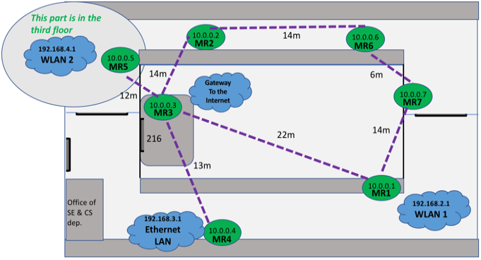 | Figure 4. OLSR-generated routes of the second topology from each mesh router to MR3 |
4.3.3. Third Topology, University Building II
The most complex topology we tested was also implemented in the same academic building and extended into the adjoining building. It was similar to the second topology with differences being the area of coverage and the location of the mesh routers which generated different routes. Figure 5 shows all of the available routes in the network as green dotted lines.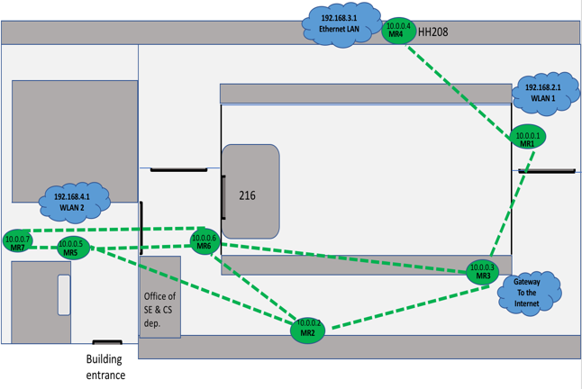 | Figure 5. Third topology consisting of seven mesh routers |
OLSR-generated routes: Figure 6 illustrates the routes generated after applying OLSR. The purple dotted lines represent the routes from each mesh router to MR3. Figure 6 shows that mesh routers MR1 and MR2 connect directly to MR3 using 1 hop, while MR4, MR6, as well as clients of the wireless LAN on MR1 are 2 hops away from MR3.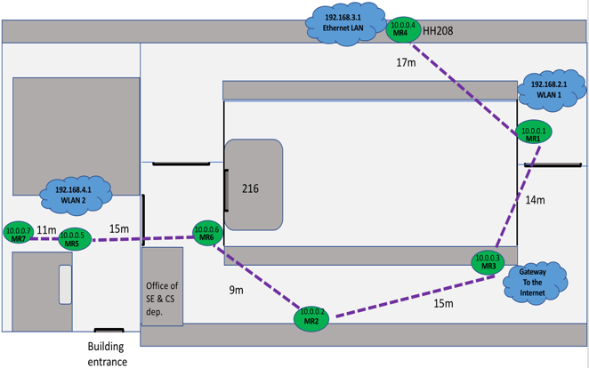 | Figure 6. OLSR-generated routes of the third topology from each mesh router to MR3 |
MR5 and clients of the Ethernet LAN on MR4 are 3 hops from MR3. Lastly, MR7 and clients of the wireless LAN on MR5 can reach MR3 through a 4-hop path. The distances from the mesh routers to MR3 are estimated and shown in Figure 6.
5. Testing and Results Analysis
5.1. Testing Approach
To evaluate the performance in our 3 topologies, we examined the following three values:1. Throughput (megabits per second): Amount of data transmitted per unit of time (seconds). 2. Jitter/delay (milliseconds): Packet delay variation which is also known as the jitter.3. Lost datagrams as a percentage of total datagrams sent: A high jitter will lead to high variations in the rate of packet arrivals at the receiver, which would lead to buffer full conditions at the receiver. This would eventually cause a loss of datagrams.The network performance testing tool we used was iperf. We installed iperf on every Raspberry Pi mesh router and also on the mesh clients of the Ethernet LAN and WLANs. The tool provides tests of TCP and UDP performance, including throughput, delay, total datagrams sent, and lost datagrams [19]. iperf uses a client/server model. To perform TCP or UDP iperf tests, we needed to run iperf on a mesh router to act as an iperf server and then run iperf on mesh nodes to make them iperf clients. In our tests, the mesh router that we used as the iperf server was MR3, the mesh router that provided Internet gateway functionality to the mesh. Figure 7 shows the output of one run of an iperf TCP test from the server and client sides. The top portion of the figure shows the client-side output, while the bottom portion shows the server-side output. The “Bandwidth” here refers to throughput. 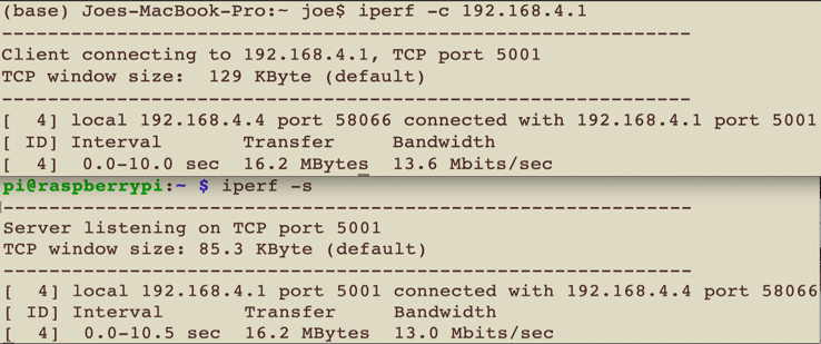 | Figure 7. Resulting output from one TCP test run of the iperf tool on the client and server sides |
Because we wanted to have a relatively large set of test data, we needed to automate the testing process using a Python script. The script ran 50 iperf TCP and UDP tests as an iperf client on each mesh router and on each client (user) of the WLANs and Ethernet LAN. The script parsed the output of each iperf run for the data that we specified and saved it to a text file. After 50 iperf runs, the script formatted the test results and saved them in the spreadsheet format shown in Figure 8.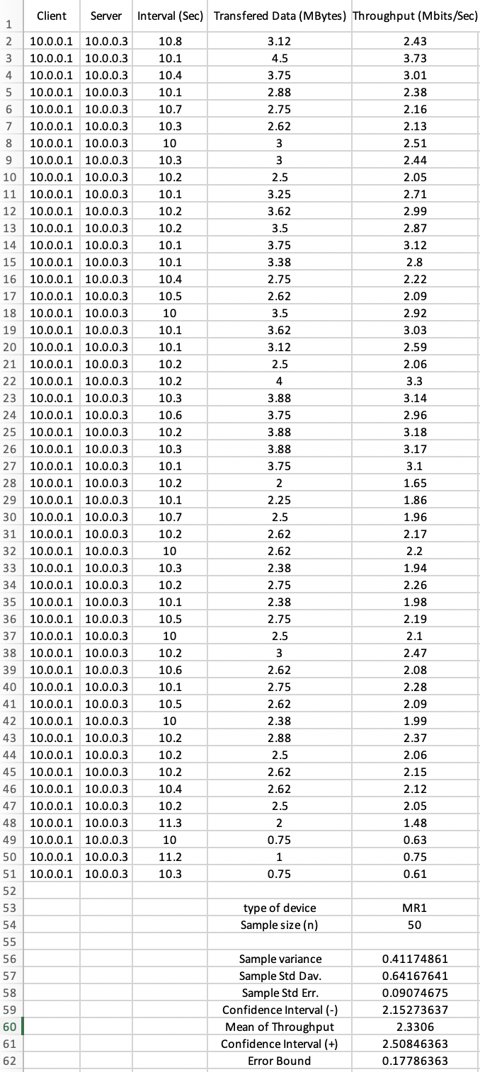 | Figure 8. Resulting data from one TCP run of our testing script |
After performing the TCP and UDP tests of the three topologies, we computed mean throughput values and applied a 95% confidence interval for the resulting TCP throughputs. For the UDP tests, we computed the mean loss of datagrams and delay/jitter. An example of the resulting test data per mesh router or client is shown in Figure 8. We have set a minimum throughput as a metric to evaluate our implemented network as a backup network access. This minimum throughput was 2 Mbps can let users keep connected and use the important services such as sharing documents, for instance, Word and Excel files and accessing the webpages.
5.2. Results
5.2.1. TCP Results
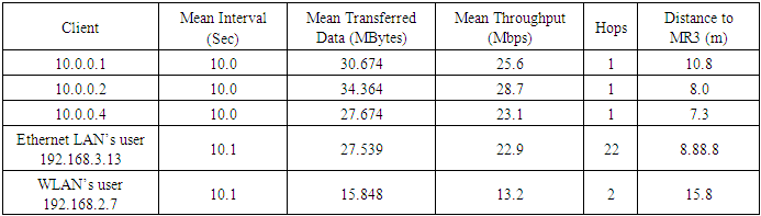
See Figures 2, 4 and 6 for the positions of mesh routers and OLSR-generated routes for the first, second, third topology, respectively. Tables 1-3 below contain the iperf client TCP test results from each mesh router and Ethernet and wireless LAN clients to the iperf server (MR3). In the tables, the “Client” column contains the IP addresses of each mesh router and the LAN clients. The mesh routers had IP addresses in the range 10.0.0.1-10.0.0.7, where the last octet is also the router’s number, e.g., 10.0.0.1 is MR1. The “Interval” column is the duration of time in seconds during which the datagrams would be transmitted. This interval includes the time until the client node receives the report from the server node, which was about half a second. The report from the server could be throughput, lost datagrams, etc. The "Hops" column represents the number of hops it takes a client to reach MR3.Table 1. First Topology TCP results with MR3 (10.0.0.3) as iperf server
 |
| |
|
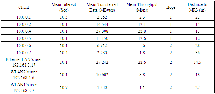
Table 2. Second topology TCP results with MR3 (10.0.0.3) as iperf server
 |
| |
|
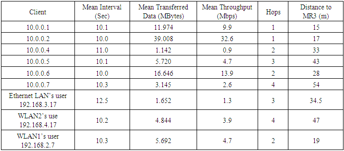
Table 3. Third topology TCP results with MR3 (10.0.0.3) as iperf server
 |
| |
|
Figures 9-11 show the resulting mean throughput per node with a 95% confidence interval. The 95% confidence interval shown in each figure is an estimation that over a range of given (sample) values, the true mean lies within that range of values, with a high degree of confidence. Using the mean and sample standard deviation, two values could be calculated: 1) the upper bound, which is the 95% maximum mean above the mean, 2) the lower bound, which is the 95% minimum mean below the mean [20]. The difference between the lower bound and the mean and the upper bound and the mean is called the error bound. In Figure 9, we show the mean of throughput that MR1 achieved with an error bound of 0.294251093. This means that we are 95% confident that the upper bound is the addition of the error bound and the mean, while the lower bound is the subtraction of the error bound from the mean.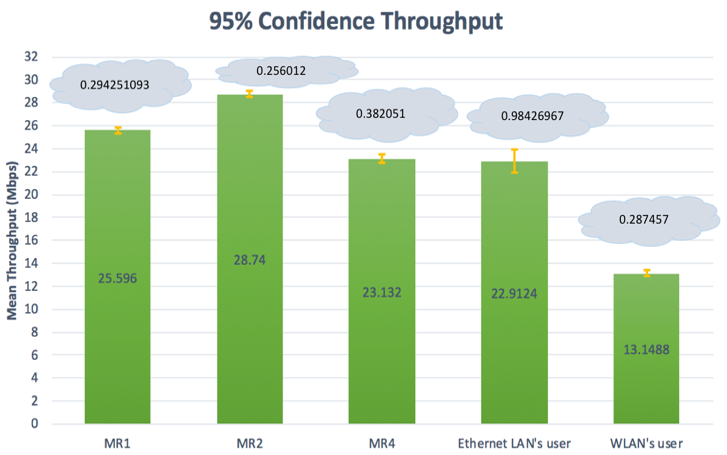 | Figure 9. First topology- Mean of throughput with a 95% confidence interval |
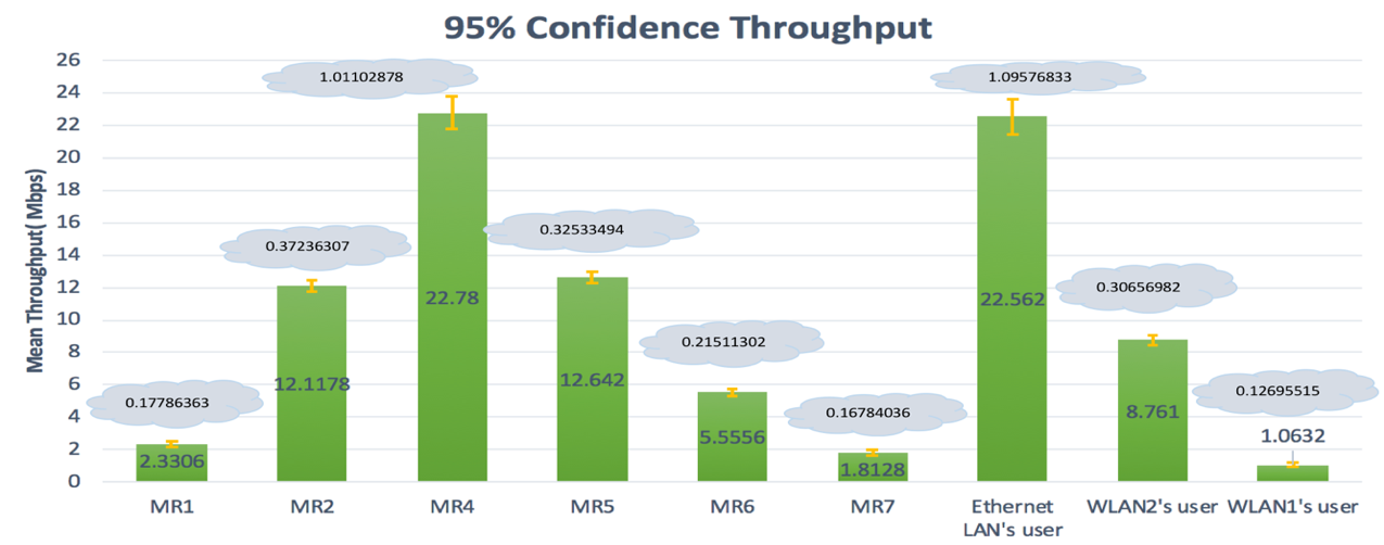 | Figure 10. Second topology- Mean of throughputs with a 95% confidence interval |
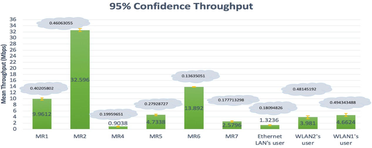 | Figure 11. Third topology- Mean of throughputs with a 95% confidence interval |
5.2.2. UDP Results
Testing UDP performance in iperf is different from testing TCP performance. We must assign some parameter values such as throughput and then send data over a set period of time to observe the delay/jitter and also the percentage of lost datagrams. In setting suitable assigned throughput values for the UDP tests, we wanted to find a maximum throughput value for a node that would still result in acceptable levels of datagram loss. Generally, the factors that increase the percentage of lost datagrams are high delay/jitter, greater transmission distance, size of receiver buffer, obstacles, and interference. The UDP results were influenced by one or more of these factors: wireless interference, physical obstacles, number of hops, and distance to MR3. To reduce UDP datagram loss, we could reduce the value of the assigned throughputs. For the first topology’s UDP tests, we assigned throughput values to each mesh router and LAN client that were greater than the mean throughputs that were measured during the TCP tests. We then measured datagram loss using iperf. In Table 4 below, the resulting values for delay/jitter and datagram loss percentage per node are shown to be within acceptable ranges for our first topology.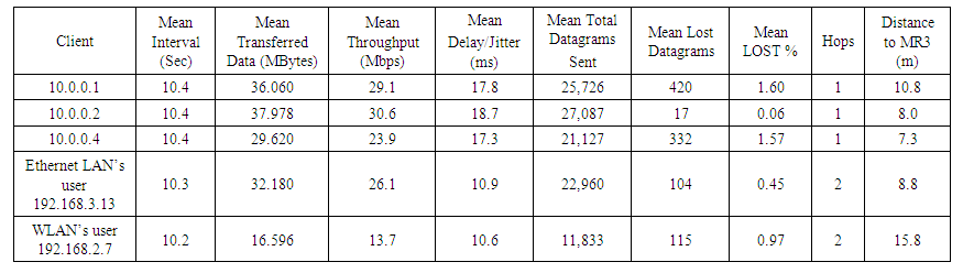 | Table 4. First topology UDP results with MR3 (10.0.0.3) as an iperf server |
As shown in Table 5 below for our second topology, in our runs of iperf on our mesh routers and LAN clients, we set a throughput value that was greater than the mean value achieved during the TCP tests, with the exceptions of MR2, MR6, and the WLAN2 client; these three were assigned 5.4, 1.5 and 8.6 Mbps, respectively. These three nodes were assigned less throughput than what they achieved in the TCP tests in order to minimize the loss of datagrams caused by the influence of long-distance, obstacles (walls), and greater wireless interference from university Wi-Fi access points along the path.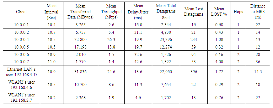 | Table 5. Second topology UDP results with MR3 (10.0.0.3) as an iperf server |
As shown in Table 6 below for our third topology, when performing the UDP tests, we assigned throughput values for the mesh routers and LAN clients that were greater than the TCP-measured throughputs, with the exception of MR7, the Ethernet client, and the WLAN2 client, all of which were 3 or more hops from MR3. For these 3 exceptions, there would have been very high UDP datagram loss if we had set throughputs equal to what was measured during the TCP tests. Table 6 shows a relationship between jitter/delay and the percentage of lost datagrams. For the Ethernet client and MR4, the assigned throughput values--1.1 and 0.9 Mbps--could not be reduced any further, which indicates that these two mesh nodes would not be usable for UDP applications that require high throughput. 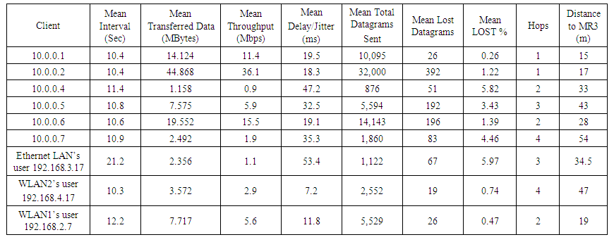 | Table 6. Third topology UDP results with MR3 (10.0.0.3) as an iperf server |
5.3. Comparison of Results
We examined and compared the best-case and worst-case measured throughputs for each of the three topologies during the iperf TCP tests.Figure 12 plots the best-achieved throughput for the 3 topologies, grouped by the number of hops to MR3. The distances to MR3 for each best-case throughput is also shown.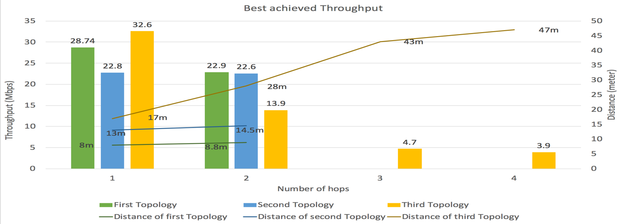 | Figure 12. Comparison of best-achieved throughput per topology |
The best-achieved throughput in the 1-hop group, 32.6 Mbps, was from the third topology; this throughput was also at the longest distance to MR3 (17 meters). In this case, the influence of distance was offset by the best-case mesh router being in line of sight with MR3. Though the best-case mesh routers for the first and second topologies were closer to MR3, both were affected by obstacles and were not in line of sight with MR3, resulting in best case throughputs of 28.74 and 22.8 Mbps.In the 2-hop group, the best-achieved throughput was 22.9 Mbps for the first topology, followed closely by 22.6 Mbps for the second topology. The Ethernet LAN client from the first topology was the best-case node, and it benefited from being just one short-distance wireless hop and one short wired hop from MR3. The Ethernet LAN client from the second topology was the second-best case node, and it also benefited from short-distance wireless and wired hops to MR3. The third topology best-case throughput, 13.9 Mbps, was achieved at a relatively long distance of 28 total meters from MR3. Only the third topology had nodes in the 3-hop and 4-hop groups, achieving 4.7 Mbps for 3 hops and 3.9 Mbps for 4 hops. Predictably, increasing the number of hops over greater distances resulted in significantly lower measured throughputs.Figure 13 plots the lowest achieved throughput for the 3 topologies, grouped by the number of hops to MR3. The distances to MR3 for each worst-case throughput is also shown.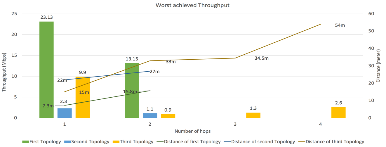 | Figure 13. Comparison of worst achieved throughput per topology |
The lowest achieved throughput in the 1-hop group, 2.3 Mbps, was from the second topology. This throughput was measured for MR1, which was located 22 meters from MR3. Though the route was only 1 hop, it was the most challenging route in terms of obstacles (Figure 4), which explains the low throughput. The worst-case throughput for the third topology was 9.9 Mbps, which is acceptable compared to the second topology. In the first topology, all node distances were relatively short, the maximum being 15.8 meters, so the worst-case measured throughput was an acceptable 23.13 Mbps.In the 2-hop group, the lowest achieved throughput was 0.9 Mbps for MR4 in the third topology due to high wireless interference, obstacles, and 33 meters total distance to MR3. The second-lowest measured throughput was 1.1 Mbps in the second topology for the WLAN1 client, which also had the worst throughput in the 1-hop group. The third lowest measured throughput was an acceptable 13.15 Mbps in the first topology at 15.8 meters to MR3. The first topology had relatively short inter-node distances and was not impacted much by obstacles.For the 3-hop and 4-hop groups, the third topology's worst-case throughputs were 1.3 Mbps at 34.6 meters and 2.6 Mbps at 54 meters from MR3, respectively. These worst-case throughputs were better than that of the second topology in the 1-hop and 2-hop cases. These worst-case throughputs were also better than the 2-hop case for the third topology, even with longer total transmission distances. The 4-hop throughput (2.6 Mbps) was also greater than the 3-hop throughput (1.3 Mbps) at a significantly greater transmission distance. This seems to indicate that the number of hops has less influence on the achieved throughput than physical obstacles, wireless interference, and total distance.The conclusion we can draw from analyzing these results is that achieved throughput for our mesh networks was impacted mainly by the presence of physical obstacles and existing wireless interference. Distance and the number of hops to a destination node seem to have less of an impact.For the purposes of a backup network, we considered 2 Mbps to be a minimum acceptable throughput. Our analysis shows that for our three pilot-scale topologies, two out of nine nodes in our second and third topologies had mean throughputs of less than 2 Mbps. Since this was a pilot-scale study, we are confident that if more MRs were added to the topologies to increase line-of-sight between nodes to avoid obstacles, then the minimum required throughput would be achieved by a larger, production-scale WMR. Acceptable performance can be achieved in a secondary backup mesh network, but the network would have to carefully designed, especially regarding node placement for obstacle avoidance and mitigation of wireless interference.
6. Conclusions
Due to its properties and relatively inexpensive implementation, a wireless mesh network could be used as a secondary, backup network in some situations such as when the main network of an organization goes down. Several studies have implemented and studied mesh networks, but most of the implemented networks used specialized networking equipment or simulation tools. We implemented low cost, pilot-scale mesh networks to evaluate feasibility as a backup network. The devices we used included Raspberry Pi’s, an Ethernet switch and several USB external Wi-Fi adapters.We implemented three topologies using the UniK-OLSR extension of the OLSR routing protocol. We tested the network performance of the topologies using the iperf tool. During the tests, which involved hundreds of runs of iperf using TCP and UDP transports, we measured three parameters from all mesh routers and mesh clients to a gateway router. The measured parameters were throughput, delay/jitter, and the percentage of lost datagrams. We used these metrics to evaluate our network and analyzed the collected data and found that the performance measures were impacted the most by obstacles and wireless interference and impacted the least by transmission distance and number of hops. The throughput measured using TCP was high for some nodes and very low in some nodes due to the positions of these nodes rather than the number of hops to the iperf server.Though the topologies that we implemented—especially the second and third topologies--all experienced significant loss of throughput, we believe that with some changes, the overall performance of our network topologies could be brought close to acceptable levels for a secondary backup network. We found that designing a mesh topology to position nodes in a way that reduces the influence of physical obstacles such as walls and interfering wireless signals would help minimize loss of inter-node throughput and would help increase the coverage area.
ACKNOWLEDGEMENTS
First, thanks to my Professor Joseph Chung for his supervision, guidelines, and support throughout the time since I started my paper up to the completion of my paper. He is a great person and brilliant professor with whom students would love to work. Fortunately, I worked with him and have been honored to work under his supervision.Second, although no words can describe how thankful to my family and friends I am, I would like to thank my family and friends who always are there for me.Lastly, special thanks to my brother and friend Ali Ghubaish for his valuable advice and notes.
References
| [1] | I. Akyildiz and X. Wang, Wireless mesh networks. Chichester, U.K.: Wiley, 2009. |
| [2] | A. Chadd, "802.11s Wireless Mesh Networking", FreeBSD 802.11, 2011. |
| [3] | V. Rastogi, V. Ribeiro, and A. Nayar, "Measurements in OLPC Mesh Networks", 2009 7th International Symposium on Modeling and Optimization in Mobile, Ad Hoc, and Wireless Networks, 2009. |
| [4] | "Wireless mesh network", En.wikipedia.org. [Online]. Available: https://en.wikipedia.org/wiki/Wireless_mesh_network. [Accessed: 28- Oct- 2017]. |
| [5] | P. Owczarek and P. Zwierzykowski, "Metrics in routing protocol for wireless mesh networks", Image Processing & Communications, vol. 18, no. 4, 2013. |
| [6] | K. Singh and S. Behal, "A Review on Routing Protocols in Wireless Mesh Networks", International Journal of Application or Innovation in Engineering & Management, vol. 2, no. 2, 2013. |
| [7] | V. Mohan.S, and K. N, "Routing Protocols for Wireless Mesh Networks", International Journal of Scientific & Engineering Research, vol. 2, no. 8, 2011. |
| [8] | K. Babu, L. Cortés-Peña, P. Shah and S. Krishnan, wi-me Wireless Mesh Network Implementation. Atlanta: School of Electrical and Computer Engineering Georgia Institute of Technology Atlanta, GA, 2007. |
| [9] | H. Yuliandoko, S. Sukaridhoto, M. Al Rasyid, and N. Funabiki, "Performance of Implementation IBR-DTN and Batman-Adv Routing Protocol in Wireless Mesh Networks", EMITTER International Journal of Engineering Technology, vol. 3, no. 1, 2015. |
| [10] | S. Bhushan, A. Saroliya and V. Singh, "Implementation and Evaluation of Wireless Mesh Networks on MANET Routing Protocols", International Journal of Advanced Research in Computer and Communication Engineering, vol. 2, no. 6, 2013. |
| [11] | D. Aguayo, J. Bicket, S. Biswas, D. De Couto and R. Morris, "MIT Roofnet Implementation", 2003. [Online]. Available: https://web.achive.org/web/20060831060307/ http://pdos.csail.mit.edu/roofnet/doku.php?id=design#overview. [Accessed: 30- Sep- 2017]. |
| [12] | G. Sims, "How to Set up a Raspberry Pi as a Wireless Access Point", MakeTechEasier, 2014. [Online]. Available: https://www.maketecheasier.com/set-up-raspberry-pi-as-wireless-access-point/. [Accessed: 10- Nov- 2017]. |
| [13] | Jacquet P., Clausen T, "Optimized Link State Routing Protocol (OLSR) ". [online] Available: https://tools.ietf.org/pdf/rfc3626.pdf [Accessed 23 Nov.2017]. |
| [14] | M. Abolhasan, B. Hagelstein, and J. Wang, "Real-world performance of current proactive multi-hop mesh protocols", 2009 15th Asia-Pacific Conference on Communications, 2009. |
| [15] | "OLSR Main Page", Olsr,org, 2016. [Online]. Available: http://www.olsr.org/mediawiki/index.php/Main_Page. [Accessed: 27- Oct- 2017]. |
| [16] | "OLSR", Staros.tog.net, 2008. [Online]. Available: http://staros.tog.net/wiki/OLSR#More_On_LinkQualityMult. [Accessed: 25- Nov- 2017]. |
| [17] | "Man page of olsrd.conf", Olsr.org, 2004. [Online]. Available: http://www.olsr.org/docs/olsrd.conf.5.html. [Accessed: 27- Nov- 2017]. |
| [18] | "servalproject/olsr", GitHub, 2012 [Online]. Available: https://github.com/servalproject/olsr/blob/master/files/olsrd.conf.default.full#L578. [Accessed: 07- Dec- 2017]. |
| [19] | "iPerf - iPerf3 and iPerf2 user documentation", Iperf.fr. [Online]. Available: https://iperf.fr/iperf-doc.php. [Accessed: 27- Nov- 2017]. |
| [20] | L. Sullivan, "Confidence Intervals", Sphweb.bumc.bu.edu. [Online]. Available: https://0x9.me/QbhM3. [Accessed: 23- Mar- 2018]. |

 Abstract
 Reference
 Full-Text PDF
 Full-text HTML