T. G. Basavaraju1, Surekha K. B.2, Mohan K. G.2
1Dept of CSE, SKSJTI, Bangalore
2Dept of CSE, ACIT, Bangalore
Correspondence to: Surekha K. B., Dept of CSE, ACIT, Bangalore.
| Email: |  |
Copyright © 2015 Scientific & Academic Publishing. All Rights Reserved.
Abstract
Wireless sensor networks are used in a wide variety of applications in our day to day life, these networks consists of small electronic devices called node or motes. These nodes will be deployed in large numbers, which are self powered, gather information or detect the required events and communicate it to the base station in a wireless mode. Sensor networks provide more number of opportunities, but at the same time pose challenge like scarcity of energy, as they have non-rechargeable batteries. As the nodes are deployed in the random fashion, due to high density of nodes, more than one node may fall in a very close proximity or in other words, two or more nodes which are very closely situated will be sensing a similar data. In this paper, we present an energy efficient routing protocol based on the closeness factor. In this approach, as soon as the deployment of the nodes is made, the base station will be grouping the set of nodes deployed in to two disjoint sets based on the closeness factor of the nodes and keep one set of nodes inactive till the other node’s energy gets depleted. Simulation results prove that lifetime of the entire network can be improved by the proposed method.
Keywords:
WSN, Non-Rechargeable, Closeness factor, Energy efficient
Cite this paper: T. G. Basavaraju, Surekha K. B., Mohan K. G., An Energy Efficient Routing Protocol Based on Closeness Factor for Wireless Sensor Networks, International Journal of Networks and Communications, Vol. 5 No. 2, 2015, pp. 31-36. doi: 10.5923/j.ijnc.20150502.02.
1. Introduction
Possible applications of sensor networks are of interest to the most diverse fields. Environmental monitoring, war-fare, child education, surveillance, micro-surgery, and agriculture are only a few examples. In ad hoc networks, wireless nodes self-organize into an infrastructure less network with a dynamic topology. Sensor networks share these traits, but also have several distinguishing features. The number of nodes in a typical sensor network is much higher than in a typical ad hoc network and dense deployments are often desired to ensure sensor area coverage and connectivity; for these reasons, sensor network hardware must be cheap. Nodes typically have less energy. Even though we assume that network will be having fixed topology, because of frequent break down of nodes, the network will be having varied topology. Life time is the critical factor for most of the applications, and energy is a major constraint in WSN’s, since a lion’s share of the energy is consumed by the operations like transmission, sensing, processing and even the hardware operation in standby mode consumes a significant amount of power as well [1].When the nodes are deployed in a geographical area, the node density may be varied from application to application, for example, the density may be as high as 20 nodes/m3 [2] or more. The redundancy of the nodes might increase the reliability level of the entire network and increase the energy consumption also. This drawback of higher density of node seen in the deployment stage can be exploited for achieving energy efficiency. To achieve the energy efficiency, it is necessary to make one set of redundant nodes to remain in energy conservation mode while the other set is in active or full power mode.In this approach, base station is responsible for separating the deployed node in to two or more disjoint sets. As soon as the deployment is done the base station will find out, which are all the nodes, which are closed to each other and it will try to separate them in to two disjoint sets. Afterwards it keeps one set of node in energy saving mode. These set of nodes remain passive until the energy of the other set nodes go down below some threshold value. Hence, the whole field will be efficiently represented by a subset of active nodes, which perform the task well. i.e. The job of sensing the data and transmitting the sensed information from the part of the geographic area is done by these subset of nodes one after the other. The experiment is conducted to study the effectiveness of the proposed mechanism.The remainder of the paper is organized as follows. Section 2 provides an overview of the existing approaches exploiting correlation. Section 3 explains the energy fundamentals of WSN. Section 4 gives proposed method. Section 5 discusses the experimental set up and results. Section 6 gives the conclusion.
2. Related Work
In this section, we discuss some of the existing approaches for achieving the energy efficiency in WSNs and improving their network lifetime [8-13]. The energy–aware immune system [3] method selects the minimum number of designated nodes that can send its data to the sink and significantly reduce the energy consumption. In addition, considering the remaining energy of the designated nodes, their energy is balanced. Hence, selecting appropriate sensors has an important effect on reducing network energy consumption and increasing its life period. By minimizing the error function, the most proper sensors for sending the data will be identified and redundancy in data sending will be eliminated.In [4], a mechanism to exploit the spatial correlation of sensor data at the link layer for event-driven WSNs is discussed and a hybrid TDMA/CSMA protocol is proposed. The protocol has three major features. First, the TDMA part is triggered only when sensors detect an event. By doing so, the protocol enjoys the benefits of collision-free transmission of TDMA and low latency transmission of CSMA. Second, the slot assignment strategy associated with the TDMA part takes the spatial correlation of sensor data into consideration. By intentionally allowing one-hop neighbors to share the same time slot, the number of slots required is significantly reduced. Thus, the transmission latency is also reduced. Third, by intentionally enlarging the slot size, packets are separated spatially and thus the interference problem in the non-event area is alleviated.In [5], since energy conservation is a key issue for WSNs, spatial correlation has been exploited; an energy aware spatial correlation based on clustering protocol is discussed. Cluster head divides the cluster in to correlation regions and in turn selects a representative node in each region. In each cycle, it chooses a representative node and only this node will be active till the end of the round, other nodes in that region will be inactive during that period. But the drawback of this method is cluster head has to waste its energy for choosing the representative node and this happens in each round.In [6], the data density correlation factor is proposed. The proposed correlation degree is a spatial correlation measurement that measures the correlation between a sensor node’s data and its neighboring sensor node’s data. With the DDCD clustering method, the sensor nodes that have high correlation are divided into the same cluster, allowing more accurate aggregated data can be obtained in cluster-based data aggregation networks produced by the DDCD clustering method. Also, the amount of data conveyed to the sink node can decrease.
3. Energy Fundamentals of WSN
The performance measure of network lifetime is particularly relevant to sensor networks where battery-powered, dispensable sensors are deployed to collectively perform a certain task. For a communication network, which is generally designed to support individual users, network lifetime is subject to interpretation; a communication network may be considered dead by one user while continuing to provide required quality of service (QoS) for others [7].In contrast, a sensor network is not deployed for individual nodes, but for a specific collaborative task at the network level. The lifetime of a sensor network thus has an unambiguous definition: it is the time span from the deployment to the instant when the network can no longer perform the task. Given that network lifetime depends on network architectures, specific applications, and various parameters across the entire protocol stack, existing techniques tend to rely on either a specific network setup or the use of upper bounds on lifetime. As such, it is difficult to develop a general design principle. Major network characteristics that affect network lifetime include network architecture, energy consumption model of sensor nodes, and data collection mode and lifetime definition determined by the underlying application [7]. Three types of sensor network architecture have been considered in the literature: flat ad hoc, hierarchical, and Sensor Network with Mobile Access (SENMA). Under the flat ad hoc architecture, sensors collaboratively relay their data to access points (in other words base stations or sinks). In hierarchical networks, sensors are organized into clusters, and cluster heads (in other words relay nodes) are responsible for collecting and aggregating data from sensors and then reporting to Access Points (APs). In SENMA, sensors communicate directly with mobile APs moving around the sensor field. Transmissions from sensors to APs are typically multi-hop in the flat ad hoc networks, single-hop in SENMA, single-hop within clusters and multi-hop between clusters in the hierarchical networks.The energy consumption model [7], characterizes the sources of energy consumption in a network. According to the rate of energy expenditure, the network energy consumption can be classified in to two general categories: the continuous energy consumption and the reporting energy consumption. The continuous energy consumption is the minimum energy needed to sustain the network during its lifetime without data collection. It includes, some of the factors like battery leakage and the energy consumed in sleeping, transition from one mode to other, sensing, and signal processing.The reporting energy consumption is the additional energy consumed in a data collection process. It depends on the channel model as well as the network architecture and protocols. In particular, the reporting energy consumption includes the energy consumed in transmission, reception, channels acquisition, collision etc.Network lifetime can be defined as the time span from the deployment to the instant when the network is considered no longer working. The decision of considering a network as nonfunctional is however, application-specific. It can be, for example, the instant when a certain fraction of sensors die, loss of coverage occurs (i.e., a certain portion of the desired area can no longer be monitored by any sensor), loss of connectivity occurs (i.e., sensors can no longer communicate with APs), or the detection probability drops below a certain threshold [7].For a highly sensitive or a critical application, the network is considered as nonfunctional soon after any one node depletes its energy. For a less sensitive application, the network is considered as functional till major set of nodes or all the nodes depletes their battery energy. Since channel states are independent of residual energies (the sensor with the better channel may have less residual energy), a lifetime-maximizing protocol needs to strike a balance between these two often conflicting objectives.
4. Proposed Method
In this section we propose a technique, in which the lifetime is improved when it is compared to a normal flat routing protocol namely DSDV. In the proposed technique, as soon as the nodes are deployed; the base station will initially gather the geographical position of every individual node. Based on the closeness factor, the nodes which are deployed are grouped in to two separate disjoint sets. The first set of nodes will be active initially during which the second set of nodes will be in the energy saving mode or in sleep mode. The reason for separating the nodes in to two disjoint sets is, when the nodes are randomly deployed, they can be anywhere in the chosen geographical area. When two or more nodes are lying nearby (very close to each other), they sense almost same information. In such cases the information will be redundant. To exploit this for energy benefit, we will find out the closeness factor between the nodes (calculate the distance between the nodes). Based on this closeness factor, divide the deployed nodes into disjoint sets. If this closeness factor is less than the threshold value, separate such nodes and maintain them in a different set.The selection of threshold value for the closeness factor is application specific and should be carefully chosen. For a highly sensitive application, for example, seismic environment, closeness factor threshold chosen must be low. But in some applications like temperature monitoring, the closeness factor threshold may be high. In other words, these nodes are more tolerant to the farthest node reporting. The closeness factor will be varying from application to application. In the simulation done, we have chosen the closeness factor threshold as 10 m. For a higher sensitive application the threshold chosen will be less than 10m. When the nodes of first set (List A) are active, the base station will monitor all the events of the sensors. The rate of data sensing of the nodes and data transmission are monitored by the Base station to track the energy level of active set of nodes. The instant at which the second set of nodes (List B) are to be activated is determined by the Base Station and in turn generates an appropriate control signal to “Turn on” the nodes of List B.
4.1. Algorithm of Proposed Method
The algorithm for grouping the deployed nodes (LTN) in to set of two disjoint sets (List A and List B) based on the closeness factor ᶿ is given below.1. Deploy the ‘n’ nodes in the specified geographic area (List of total nodes LTN), the nodes are deployed in random fashion.2. Each node is represented by its X and Y coordinate e.g. ith node is represented as Ni(Xi, Yi) and all the nodes are initially active.3. Get the geographical position of each individual node in to the Base Station and copy the list of the total nodes LTN in to List A.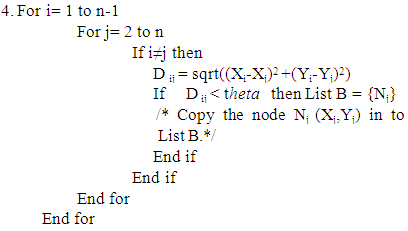 5. All the nodes of list B are set to power saving mode or turned off, keeping the nodes of list A in the active state.
5. Experimental Set up and Results
The performance of the above proposed model is evaluated by using ns-2 simulator. The performance result of the proposed mechanism is compared with the normal flat routing protocol. In the simulation, node deployment area was considered as an area of 100 m X 100 m. Initial energy of every node is assumed as 10 Joules. The closeness factor threshold theta is assumed as 10 m. The simulation parameters assumed are given in the Table 1.| Table 1. Simulation parameters |
| | Variables | Values | | RX Power | 0.00175W | | TX Power | 0.00175W | | Initial energy of every node | 10 J | | Sleep Power | 0.0005W | | Transition Power | 0.002W |
|
|
To analyze the performance of the proposed method, we have considered two issues namely Coverage and Network lifetime.Initially, all 100 nodes were set in normal mode ‘on’, and performance is evaluated. Even though, it is felt that, the proposed method is going to utilize the resources efficiently, if the set of some nodes did not cover the entire network area then it is of no use if the resources are saved. So, the area coverage by the nodes of the normal flat routing protocol is compared with the proposed method. Figure 1 shows the deployment of nodes in list LTN. The deployment of the node is in random fashion. After applying the proposed method the LTN is grouped in to two sets. Distribution of the List A nodes in the simulation area is shown in Figure 2. Similarly List B nodes distribution is shown in Figure 3.One of the parameter chosen to find out the effectiveness of the proposed mechanism is the coverage of the area by the nodes deployed. The coverage of the area by the nodes in normal flat routing protocol is considered as 100%. In the proposed mechanism, the total deployed nodes are grouped in to two separate lists. The coverage of the area by the distribution pattern of the nodes of List A and List B are determined and normalized to the area coverage of normal flat routing protocol. 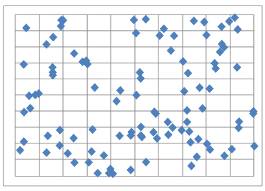 | Figure 1. Plot showing the position of all the nodes deployed for scenario 1 |
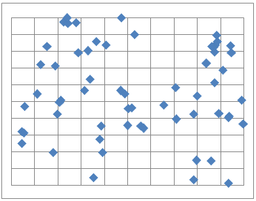 | Figure 2. Plot showing the position of List A the nodes deployed for Scenario 1 |
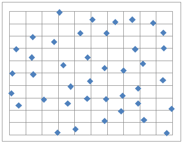 | Figure 3. Plot showing the position of List B nodes deployed for Scenario 1 |
In Figure 4, the network area coverage for 100 nodes for five different scenarios is shown. From figure 4, it is observed that, area coverage using normal flat routing protocol is 100%, for the List A nodes, coverage area is 93%. From the List B nodes 91% coverage is seen. Simulation is done for five different scenarios and results are included in figure 4. On an average of 94% coverage can be seen with the proposed method. By this a conclusion can be made, even though a set of nodes are turned off, the coverage is almost equal to the normal flat routing protocol. Table 2 and Table 3 shows the number of nodes which are in List A and List B. Similarly Figure 5 shows the area coverage by total 150 nodes for five different scenarios.| Table 2. Number of Nodes which fall in to List A & B out of 100 |
| | Nodes list | *Sc 1 | Sc 2 | Sc 3 | Sc 4 | Sc 5 | | LTN | 100 | 100 | 100 | 100 | 100 | | LIST A | 60 | 56 | 54 | 60 | 54 | | LIST B | 40 | 44 | 46 | 40 | 46 | | *Sc 1 : Scenario 1 |
|
|
| Table 3. Number of nodes which fall into List A & B out of 150 |
| | Nodes list | Sc1 | Sc2 | Sc3 | Sc 4 | Sc5 | | LTN | 150 | 150 | 150 | 150 | 150 | | LIST A | 106 | 100 | 103 | 102 | 103 | | LIST B | 44 | 50 | 47 | 48 | 49 |
|
|
Another parameter chosen to prove the effectiveness of the proposed mechanism is the network life time. The network life time was measured and is compared with the normal flat routing protocol. In this experiment, we have considered network lifetime as time span from the start till any node losses its battery power completely. In Figure 6, the network lifetime using flat routing protocol and the proposed mechanism for five different scenarios is shown. For the first scenario, the network life time for normal flat routing protocol is 11.716s, i.e. the time at which the first node died. In the proposed method, when the List A nodes were ‘on’, the lifetime was measured as 10.94 s, i.e, when the first node died and the instant at which the second set of nodes(List B) were turned ‘on’. The lifetime of the List B nodes was measured as 11.637s after the first node of List A died. Together if it is considered, the total life time in proposed method is 22.557s for the first scenario. For the proposed mechanism, the average network lifetime for five different scenarios is 21s. In the Figure 7, results are shown for 150 nodes.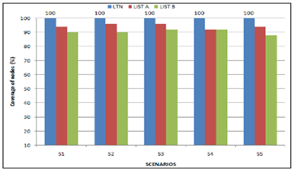 | Figure 4. Coverage of simulation area for 100 nodes |
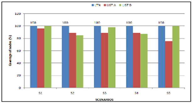 | Figure 5. Coverage of simulation area for 150 nodes |
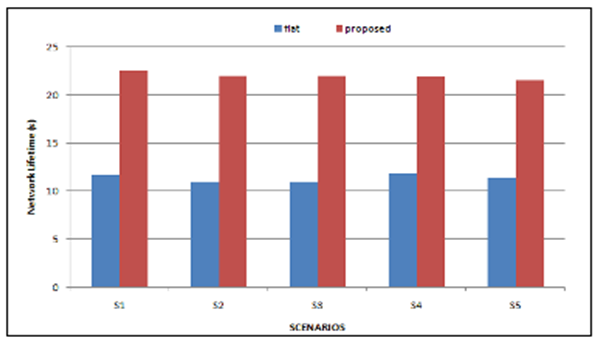 | Figure 6. Lifetime for 100 nodes |
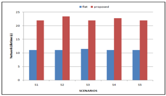 | Figure 7. Lifetime for 150 nodes |
The network lifetime measured was almost doubled in the proposed method.
6. Conclusions
As the energy is the major resource constraint in WSN, energy efficient routing protocols are to be designed. The aim of designing routing protocols is to be saving the energy and improving the network lifetime. In this proposed technique a method to improve the network lifetime is discussed. Among the deployed nodes, the nodes will be divided in to two different sets based on the closeness factor. The first set nodes will be turned on initially, and when the energy of the any one node in the first set is nearing to zero, we turn on the second set of nodes, which were earlier in the sleeping mode. The proposed method is compared with existing method; the network lifetime is increased nearing to 100%. With the proposed method, the coverage is also maintained to the average to 94%. As a future work, the same technique can be extended to hierarchical routing protocols also.
References
| [1] | Daniele Puccinelli and Martin Haenggi “Wireless sensor networks: applications and challenges of ubiquitous sensing” IEEE Circuits and Systems Magazine, Volume 5, Issue 3, 2005, pp 19-31. |
| [2] | C. Intanagonwiwat, R. Govindan, and D. Estrin, “Directed Diffusion: a Scalable and Robust Communication Paradigm for Sensor Networks,” in Proc ACM MobiCOM 2000, Boston, MA, 2000, pp. 56-67. |
| [3] | Samira Nemati, Reza Azmi and M.A.S monfared, An Energy aware Spatial Correlation Method in Event driven Wireless Sensor Networks, IJCSI International Journal of Computer Science Issues, Vol. 9, Issue 5, No 3, September 2012 ISSN (Online): 1694-0814. |
| [4] | Chih-Yu-Lin, Yu-Chee Tseng, Ten H. Lai, Exploiting Spatial Correlation at the Link Layer for Event-driven Sensor Networks, International Journal of Sensor Networks,2012 Vol. 12, No 1, pp 1-15. |
| [5] | Ghalib A. Shah and Muslim Bozyigit Exploiting Energy-aware Spatial Correlation in Wireless Sensor Networks, in Proc. Communication System Software and Middleware, COMSWARE, 2007, IEEE. |
| [6] | Fei Yuan; Sch. Of Inf. Sci. & Technol., Sun-Yat Sen Univ., Guangzo, China; Yiju Zhan; Yonghua Wang Data Density Correlation Degree Clustering Method for Data Aggregation in WSN, Sensors Journal Volume 14 Issue 4, IEEE Sensor Council 2014. |
| [7] | Edited by Ananthram Swami Army Research Laboratory, USA Qing Zhao, Yao-Win Hong, Lang Tong Wireless Sensor Networks Signal Processing and Communications Perspectives, Wiley International, 2007. |
| [8] | M. G. C. Torres, “Energy consumption in wireless sensor networks using GSP,” M.S. dissertation, Universiy of Pittsburgh, 2006. |
| [9] | Min Yao, Chuang Lin, Peng Zhang, Yuan Tian, Shibo Xu, “TDMA scheduling with maximum throughput and Fair Rate Allocation in Wireless Sensor Networks” in Proc IEEE,ICC 2013,Adhoc and Sensor Networking symposium. |
| [10] | W. R. Heinzelman, A. Chandrakasan, and H. Balakrishnan, “Energy Efficient Communication Protocol for Wireless Microsensor Networks,” In Proceedings of the 33rd Hawaii International Conference on System Sciences-2000, pp. 3005–3014, 2000. |
| [11] | M. C. Vuran, O. B. Akan, and I. F. Akyildiz, “Spatio-temporal correlation: theory and applications for wireless sensor networks,” Computer Network. J. (Elsevier), vol. 45, pp. 245–259, 2004. |
| [12] | Shakya R.K; Singh N; Verma N K. A novel spatial correlation model for wireless sensor network applications Wireless and Optical Communications Networks (WOCN), 2012 Ninth International Conference. |
| [13] | W. Heinzelman, A. Chandrakasan, and H. Balakrishnan, “Energy Efficient Routing Protocols for Wireless Microsensor Networks,” in Proc. 33rd Hawaii International Conference on System Sciences (HICSS ’00), Jan. 2000. |
 Abstract
 Reference
 Full-Text PDF
 Full-text HTML