1. Introduction

The well-known QR codes, introduced by Prange[1] in 1957, are cyclic BCH codes with code rates greater than or equal to one-half. In addition, the codes generally have large minimum distances so that most of the known QR codes are the best-known codes. The code augmented by a parity bit, for example, the (24, 12, 8) QR code was utilized to provide error control on the Voyager deep-space mission[2].

In the past decades, several decoding techniques have been developed to decode the binary QR codes. The ADAs most used to decode the QR codes are the Newton identities with either Sylvester resultants[3-7,12-13,15] or Gröbner bases[16] , or inverse-free Berlekamp-Massey (IFBM) algorithm[8-11,14] to determine the error-locator polynomial. Among them, the ADA of the (31, 16, 7) QR code[5,12,14,15] with the reducible polynomial can correct up to three errors in the finite field GF(2⁵), because the error-correcting capability of the code is errors, where denotes the greatest integer less than or equal to x, and d = 7 is the minimum Hamming distance of the code. In[5,12,15], the Newton identities are applied to determine the coefficients of the error-locator polynomials. In[14], the IFBM algorithm[18] is applied to determine the error-locator polynomial of the received sequence. Finally, the Chien search algorithm[19] is applied to find the roots of the error-locator polynomial.

In[15], the decoding algorithm is very complicated because the syndrome S₇ = 0. However, the IFBM does not use the syndrome S₇ to determine the error-locator polynomial of the (31, 16, 7) QR code. For the QR codes with irreducible generator polynomial, the primary known syndrome S₁ cannot be equal to zero, because the zero S₁ denotes that the received word has no errors in the transmission channel. Besides, S₁ = 0 means that the power (mod codelength n) of S₁ are all zero; that is, S₂ = (S₁)² = 0, S₄ = (S₁)⁴ = 0, …. For the (89, 45, 17) QR code with reducible generator polynomial in the finite field GF(2¹¹), the IFBM algorithm can be used to determine the error-locator polynomial while the syndrome S₁ = 0[20]. Similarly, for the (31, 16, 7) QR code with reducible generator polynomial in the finite field GF(2⁵), the zero primary known syndromes, S₁ = 0 and S₅ = 0, do not cause a decoding failure in decoding weight-3 error patterns while using the IFBM algorithm to determine the error-locator polynomial. The analysis of two examples on the weight-3 error patterns shows the fact.

The rest parts of this paper are organized as follows: The background of systematic (31, 16, 7) QR codes is briefly given in Section 2. The analysis on the zero primary known syndromes for the weight-3 error patterns is presented in Section 3. Finally, this paper concludes with a brief summary in Section 4.

2. Background of the Binary (31, 16, 7) QR Code

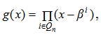
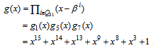
The codeword of the binary (n, k, d) QR code is defined algebraically as a multiple of its generator polynomial g(x) with coefficients in GF(2). Let the length of the code n be a prime number of the form n = 8m ± 1, where m is a positive integer and m be the smallest positive integer such that 2^m ≡ 1 (mod n). Thus, GF(2^m) is the extension field of GF(2). Also, let k = (n+1)/2 be the message length and d be the minimum Hamming distance or Hamming weight of the code. The generator polynomial as a cyclic code is given by

(1)

where the element β is a primitive nth root of unity in GF(2^m) and Q_n denotes the set of quadratic residues given by Q_n = {jj ≡ x² mod n for 1 ≤ x ≤ (n–1)/2}. The set Q_n can thus be represented as a disjoint union of cyclotomic cosets, modulo n. These cyclotomic cosets are defined as Q_r = {r2^jj = 0, 1, … , n_r–1}, where n_r is the smallest positive integer such that , n_r divides (n–1)/2, and r is the smallest element in Q_r. The element r is called the representative element of the cyclotomic cosets Q_r. The set S, consisting of all representatives of the QR code, is called the base set of the QR code. 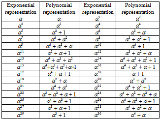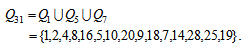These definitions and properties cause the equality relating Q_n to the cyclotomic cosets, modulo n.

Let an element α GF(2⁵) be a root of the primitive polynomial p(x) = x⁵ + x² + 1. Then, α generates the multiplicative group of nonzero elements in GF(2⁵). Also, let an element β = α^u, where u = (2^m – 1)/n = (2⁵ – 1)/31 = 1, is a primitive 31th root of unity in GF(2⁵); that is, β = α. The all 31 roots of x³¹ – 1 = 0 are shown in Table 1.

Table 1. The 31 Roots of x31 – 1 = 0

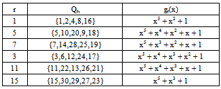
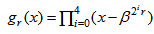The base set of this code is S = {1, 5, 7, 3, 11, 15} and r ∈ S. The minimal polynomial g_r(x) can also be expressed as . Therefore, the six cyclotomic cosets Q_r and their corresponding minimal polynomials are shown in Table 2.

Table 2. The Cyclotomic Cosets of the (31, 16, 7) QR Code

Let r = 1, 5, and 7, respectively, the quadratic residue set of the code is

(2)

Thus, the g(x) consists of the following three minimum polynomials:

(3)

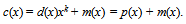
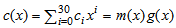Since the codewords are a multiple of the g(x), the codeword polynomial of the (31, 16, 7) QR code can be represented by , where c_i ∈ GF(2) for 0 ≤ i ≤ 30, and m(x) = m₁₅x¹⁵ + + m₁x + m₀ denotes information polynomial, where m_i ∈ GF(2) for 0 ≤ i ≤ 15. In such a representation, this type of codeword is called the non-systematic encoding. In practice, the encoding procedure is often implemented by the use of systematic encoding. Let p(x) = p₁₄x¹⁴ + + p₁x + p₀ be the parity-check polynomial, where p_i ∈ GF(2) for 0 ≤ i ≤ 14. Also, let m(x)x^n-k divide by g(x), then we get the following identity:

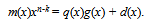(4)

Multiplying both sides of (4) by x^k and using xⁿ = 1, Then, it yields d(x)x^k + m(x) = (q(x)x^k)g(x). The term d(x)x^k + m(x), which is a multiple of g(x), has m(x) in its lower k bits and p(x) = d(x)x^k in its higher n – k bits. Thus, the codeword can be represented by the equation below.

(5)

As shown in (5), this form of the codeword is called systematic encoding. Now, let a codeword be transmitted through a noisy channel to obtain a received word of the form r(x) = c(x) + e(x), where e(x) = e₃₀x³⁰ ++ e₁x + e₀ is the occurred error polynomial and e_i ∈ GF(2). For simplification, the polynomial form can be expressed as the vector form. For example, c(x) can be expressed as c = (c₃₀, …, c₁, c₀). The syndromes or known syndromes of the code are defined by

(6)

where i (mod 31) ∈ Q₃₁. If i ∉ Q₃₁, the syndromes are called unknown syndromes. All known and unknown syndromes can be expressed as some powers of S₁, S₅, S₇, and S₃, S₁₁, S₁₅, called the primary known syndromes and the primary unknown syndromes, respectively. For example, S₂ = S₁², S₄ = S₁⁴, S₈ = S₁⁸, and S₁₆ = S₁¹⁶. Note that S₀ = 0 or 1 depends on the fact that v is even or odd, where v is the actual number of errors to be corrected and 1 ≤ v ≤ 3.

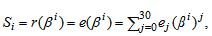
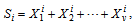If there are v ≤ t errors in r(x), then e(x) has v nonzero terms over GF(2); that is,, where 0 ≤ r₁ < r₂ < ... < r_v ≤ n–1. For i ∈ Q_n, the syndrome can be written as where for 1 ≤ j ≤ v are called the error locators. Assuming that v errors occur, the classical error-locator polynomial L(x) is defined by

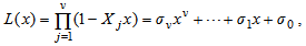(7)

where the σ_j are called the elementary symmetric functions for 1 ≤ j ≤ v and σ₀ = 1. The roots of L(x) are the inverse of the v error locators {X_j}.

The steps of the IFBM algorithm are summarized as below:

1).Initialize k = 0, μ⁽⁰⁾(x) = 1, λ⁽⁰⁾(x)=1, l⁽⁰⁾ = 0, γ⁽⁰⁾ = 1.

2).Compute

(8)

where μ_j^(k–1) is the coefficient of μ^(k–1)(x).

3).Compute

(9)

4).Compute

(10)

5).Set k = k + 1. If k ≤ 2t, then go to step 2. Otherwise go to stop and declare a decoding failure.

3. Analysis on the Zero Primary Known Syndromes for the Weight-3 Error Patterns

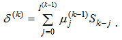
The ADA given in[14] used the IFBM algorithm to determine the error-locator polynomial. In order to use the IFBM algorithm, the consecutive syndromes, Si for 1 ≤ i ≤ 6, need to be computed first. Among them, there are two unknown syndromes S3, and S6, where S6 can be computed from the square of S3. The determination of the unknown syndrome S3 is computed from (17) of[12].

For the (31, 16, 7) QR code, a C++ program shows that there are 155 weight-3 error patterns will cause the primary known syndromes and the primary unknown syndromes to be equal to zero; however, they are not simultaneous equal to zero. The zero primary known syndromes do not cause a decoding failure while using the IFBM algorithm to determine the error-locator polynomial. The following example shows the decoding procedure.

3.1. The Case of Primary Known Syndrome S₁ = 0

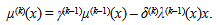
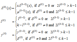
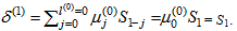
Example 1:

If m(x) = x⁷, by (4) and (5), then the systematic codeword is c(x) = x³⁰ + x²⁹ + x²⁷ + x²⁶ + x²⁵ + x²⁰ + x¹⁹ + x⁷. If there is a weight-3 error pattern e(x) = x¹⁸ + x + 1 occurred in the transmission channel, then the received word becomes r(x) = x³⁰ + x²⁹ + x²⁷ + x²⁶ + x²⁵ + x²⁰ + x¹⁹ + x¹⁸ + x⁷ + x + 1.

The syndromes S₁ = 0, S₂ = 0, S₄ = 0, and S₅ = α³⁰ are computed by (6), respectively, and the syndromes S₃ = α¹⁹ and S₆ = S₃² = α⁷ are computed by (17) in[12]. Next, the IFBM algorithm is applied to obtain the error-locator polynomial. The decoding procedure is described as follows:

Define initial value as follows: k = 0, μ⁽⁰⁾(x) = 1, λ⁽⁰⁾(x)=1, l⁽⁰⁾ = 0, γ⁽⁰⁾ = 1.

Set k = k + 1 = 0 + 1 = 1. By (8), compute

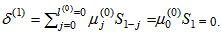By (9), compute μ⁽¹⁾(x) = γ⁽⁰⁾μ⁽⁰⁾(x) – δ⁽¹⁾λ⁽⁰⁾(x)•x = 1∙1 – 0∙1∙x = 1.

The condition in (10) is δ⁽¹⁾ = 0. Compute λ⁽¹⁾(x) = xλ⁽⁰⁾(x) = x, l⁽¹⁾ = l⁽⁰⁾ = 0, and γ⁽¹⁾ =γ⁽⁰⁾ = 1, respectively. Go to step 2.

Set k = k + 1 = 1 + 1 = 2. By (8), compute

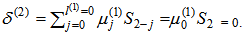By (9), compute μ⁽²⁾(x) = γ⁽¹⁾μ⁽¹⁾(x) – δ⁽²⁾λ⁽¹⁾(x)x = 0∙1 – 0∙1∙x = 1.

The condition in (10) is δ⁽²⁾ = 0. Compute λ⁽²⁾(x) = xλ⁽¹⁾(x) = xx = x², l⁽²⁾ = l⁽¹⁾ = 0, and γ⁽²⁾ = γ⁽¹⁾ = 1, respectively. Go to step 2.

Set k = k + 1 = 2 + 1 = 3. By (8), compute

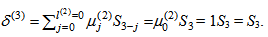By (9), compute μ⁽³⁾(x) = γ⁽²⁾μ⁽²⁾(x) – δ⁽³⁾λ⁽²⁾(x)•x = 1∙1 – S₃∙x²∙x = 1 + S₃x³.

The conditions in (10) are δ⁽³⁾ = S₃ ≠ 0 and 2l⁽²⁾ = 0 ≤ k – 1 = 3 – 1 = 2. Compute λ⁽³⁾(x) = μ⁽²⁾(x) = 1, l⁽³⁾ = k - l⁽²⁾ = 3 – 0 = 3, and γ⁽³⁾ = δ⁽³⁾ = S₃, respectively. Go to step 2.

Set k = k + 1 = 3 + 1 = 4. By (8), compute.

By (9), compute μ⁽⁴⁾(x) = γ⁽³⁾μ⁽³⁾(x) – δ⁽⁴⁾λ⁽³⁾(x)•x = S₃(1 – S₃x³) = S₃ + S₃²x³.

The condition in (10) is δ⁽⁴⁾ = 0. Compute λ⁽⁴⁾(x) = x•1 = x, l⁽⁴⁾ = l⁽³⁾ = 3, and γ⁽⁴⁾ = γ⁽³⁾ = S₃, respectively. Go to step 2.

Set k = k + 1 = 4 + 1 = 5. By (8), compute

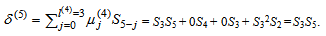By (9), compute the error-locator polynomial of degree 3, μ⁽⁵⁾(x) = γ⁽⁴⁾μ⁽⁴⁾(x) – δ⁽⁵⁾λ⁽⁴⁾(x)•x = S₃(S₃ + S₃²x³) – (S₃S₅)xx = S₃² + S₃S₅x² + S₃³x³.

The condition in (10) is 2l^(k-1) = 2l⁽⁴⁾ = 6 > k – 1 = 5 – 1 = 4. Compute λ⁽⁵⁾(x) = xλ⁽⁴⁾(x) = xx = x², l⁽⁵⁾ = l⁽⁴⁾ = 3, and γ⁽⁵⁾ = γ⁽⁴⁾ = S₃, respectively. Go to step 2.

Set k = k + 1 = 5 + 1 = 6. By (8), compute

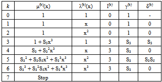
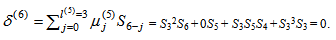By (9), compute the error-locator polynomial of degree 3, μ⁽⁶⁾(x) = γ⁽⁵⁾μ⁽⁵⁾(x) – δ⁽⁶⁾λ⁽⁵⁾(x)x = S₃(S₃² + S₃S₅x² + S₃³x³) = S₃³ + S₃²S₅x² + S₃⁴x³.

The condition in (10) is δ⁽⁶⁾ = 0, compute λ⁽⁶⁾(x) = xλ⁽⁵⁾(x) = xx² = x³, l⁽⁶⁾ = l⁽⁵⁾ = 3, and γ⁽⁶⁾ = γ⁽⁵⁾ = S₃, respectively. Go to step 2.

Set k = k + 1 = 6 + 1 = 7. Since k = 7 > 2t = 6, go to stop.

The above decoding procedure is simplified in Table 3.

Table 3. The Simplified Decoding Procedure for Example 1

When k = 6, one obtains the error-locator polynomial μ⁽⁶⁾(x) = L(x) = S₃³ – S₃²S₅x² – S₃⁴x³, which means that μ⁽⁶⁾(x) has three roots. By applying Chien search algorithm, the roots of L(x) are exactly the inverse of the three error locators {0, 1, 18}. For example, the third error locator is α¹⁸, and the reciprocal of α¹⁸ is α¹³. Substituting α¹³ into L(x), then the error-locator polynomial L(α¹³) = S₃³ + S₃²S₅(α¹³)² + S₃⁴(α¹³)³ = (α¹⁹)³ + (α¹⁹)²(α³⁰)(α¹³)² + (α¹⁹)⁴(α¹³)³ = α²⁶ + α + α²² = 0. Similarly, the first and the second error locators are α⁰ and α¹, then we obtain L(1) = 0 and L(α³⁰) = 0, respectively. A C++ program shows that the total 155 weight-3 error patterns with S₁ = 0 can be corrected.

3.2. The Case of Primary Known Syndrome S₅ = 0

Example 2:

If m(x) = x⁷, by (4) and (5), then the systematic codeword is c(x) = x³⁰ + x²⁹ + x²⁷ + x²⁶ + x²⁵ + x²⁰ + x¹⁹ + x⁷. If there is a weight-3 error pattern e(x) = x¹⁹ + x + 1 occurred in the transmission channel, then the received word becomes r(x) = x³⁰ + x²⁹ + x²⁷ + x²⁶ + x²⁵ + x²⁰ + x⁷ + x + 1.

The known syndromes S₁ = α⁵, S₂ = α¹⁰, S₄ = α²⁰, and S₅ = 0 are computed by (6), respectively, and the known syndromes S₃ = α²⁴ and S₆ = α¹⁷ are computed by (17) in[12]. Next, the IFBM algorithm is applied to obtain the error-locator polynomial. The decoding procedure is described as follows:

Define initial value as follows: k = 0, μ⁽⁰⁾(x) = 1, λ⁽⁰⁾(x)=1, l⁽⁰⁾ = 0, γ⁽⁰⁾ = 1.

Set k = k + 1 = 0 + 1 = 1. By (8), compute

By (9), compute μ⁽¹⁾(x) = γ⁽⁰⁾μ⁽⁰⁾(x) – δ⁽¹⁾λ⁽⁰⁾(x)•x = 1∙1 – S₁∙1∙x = 1 + S₁x.

By (10), the conditions δ⁽¹⁾ = S₁ ≠ 0 and 2l⁽⁰⁾ = 2∙0 = 0 ≤ k – 1 = 1 – 1 = 0 are satisfied. Then compute λ⁽¹⁾(x) = μ⁽⁰⁾(x) = 1, l⁽¹⁾ = k – l⁽⁰⁾ = 1 – 0 = 1, and γ⁽¹⁾ = δ⁽¹⁾ = S₁, respectively. Go to step 2.

Set k = k + 1 = 1 + 1 = 2. By (8), compute

By (9), compute μ⁽²⁾(x) = γ⁽¹⁾μ⁽¹⁾(x) – δ⁽²⁾λ⁽¹⁾(x)x = S₁(1 + S₁x) – 0∙1∙x = S₁ + S₁²x.

By (10), the condition δ⁽²⁾ = 0 is satisfied. Then compute λ⁽²⁾(x) = xλ⁽¹⁾(x) = x, l⁽²⁾ = l⁽¹⁾ = 1, and γ⁽²⁾ = γ⁽¹⁾ = S₁, respectively. Go to step 2.

Set k = k + 1 = 2 + 1 = 3. By (8), compute

By (9), compute μ⁽³⁾(x) = γ⁽²⁾μ⁽²⁾(x) – δ⁽³⁾λ⁽²⁾(x)•x = S₁(S₁ + S₁²x) – (S₁S₃ + S₁⁴)∙x∙x = S₁² + S₁³x +(S₁S₃ + S₁⁴)x².

By (10), the conditions δ⁽³⁾ ≠ 0 and is 2l⁽²⁾ = 2 ≤ k – 1 = 3 – 1 = 2. Compute λ⁽³⁾(x) = μ⁽²⁾(x) = S₁ + S₁²x, l⁽³⁾ = k – l⁽²⁾ = 3 – 1 = 2, and γ⁽³⁾ = δ⁽³⁾ = S₁S₃ + S₁⁴, respectively. Go to step 2.

Set k = k + 1 = 3 + 1 = 4. By (8), compute. 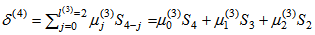= S₁²S₄ + S₁³S₃ + (S₁S₃ + S₁⁴)S₂ = 0.

By (9), compute μ⁽⁴⁾(x) = γ⁽³⁾μ⁽³⁾(x) – δ⁽⁴⁾λ⁽³⁾(x)•x = (S₁S₃ + S₁⁴)( S₁² + S₁³x +(S₁S₃ + S₁⁴)x²) – 0(S₁ + S₁²x)x = (S₁³S₃ + S₁⁶) + (S₁⁷ + S₁⁴S₃)x + (S₁²S₃² + S₁⁸)x².

By (10), the condition in is δ⁽⁴⁾ = 0 is satisfied. Then compute λ⁽⁴⁾(x) = xλ⁽³⁾(x) = x(S₁ + S₁²x) = S₁x + S₁²x², l⁽⁴⁾ = l⁽³⁾ = 2, and γ⁽⁴⁾ = γ⁽³⁾ = S₁S₃ + S₁⁴, respectively. Go to step 2.

Table 4. The Simplified Decoding Procedure for Example 2

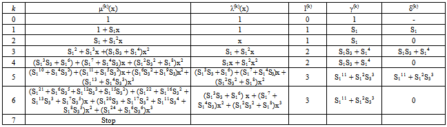
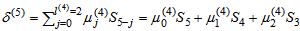Set k = k + 1 = 4 + 1 = 5. By (8), compute = (S₁³S₃ + S₁⁶)0 + (S₁⁷ + S₁⁴S₃)S₄ + (S₁²S₃² + S₁⁸)S₃ = S₁¹¹ + S₁²S₃³.

By (9), compute μ⁽⁵⁾(x) = γ⁽⁴⁾μ⁽⁴⁾(x) – δ⁽⁵⁾λ⁽⁴⁾(x)•x = (S₁S₃ + S₁⁴)((S₁³S₃ + S₁⁶) + (S₁⁷ + S₁⁴S₃)x + (S₁²S₃² + S₁⁸)x²) – (S₁¹¹ + S₁²S₃³)(S₁x + S₁²x²)x = (S₁¹⁰ + S₁⁴S₃²) + (S₁¹¹ + S₁⁵S₃²)x + (S₁⁶S₃² + S₁⁹S₃)x² + (S₁¹³ + S₁⁴S₃³)x³.

By (10), the conditions δ⁽⁴⁾ ≠ 0 and 2l^(k-1) = 2l⁽⁴⁾ = 4 ≤ k – 1 = 5 – 1 = 4 are satisfied. Then compute λ⁽⁵⁾(x) = μ⁽⁴⁾(x) = (S₁³S₃ + S₁⁶) + (S₁⁷ + S₁⁴S₃)x + (S₁²S₃² + S₁⁸)x², l⁽⁵⁾ = k – l⁽⁴⁾ = 5 – 2 = 3, and γ⁽⁵⁾ = δ⁽⁵⁾ = S₁¹¹ + S₁²S₃³, respectively. Go to step 2.

Set k = k + 1 = 5 + 1 = 6. By (8), compute δ^{(6) =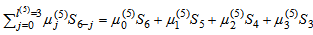} = (S₁¹⁰ + S₁⁴S₃²)S₆ + (S₁¹¹ + S₁⁵S₃²)S₅ + (S₁⁶S₃² + S₁⁹S₃)S₄ + (S₁¹³ + S₁⁴S₃³)S₃ = 0.

By (9), compute the error-locator polynomial of degree 3, μ⁽⁶⁾(x) = γ⁽⁵⁾μ⁽⁵⁾(x) – δ⁽⁶⁾λ⁽⁵⁾(x)x = (S₁¹¹ + S₁²S₃³)( (S₁¹⁰ + S₁⁴S₃²) + (S₁¹¹ + S₁⁵S₃²)x + (S₁⁶S₃² + S₁⁹S₃)x² + (S₁¹³ + S₁⁴S₃³)x³) – 0((S₁³S₃ + S₁⁶) + (S₁⁷ + S₁⁴S₃)x + (S₁²S₃² + S₁⁸)x²)x = (S₁²¹ + S₁⁶S₃⁵ + S₁¹²S₃³ + S₁¹⁵S₃²) + (S₁²² + S₁¹⁶S₃² + S₁¹³S₃³ + S₁⁷S₃⁵)x + (S₁²⁰S₃ + S₁¹⁷S₃² + S₁¹¹S₃⁴ + S₁⁸S₃⁵)x² + (S₁²⁴ + S₁⁶S₃⁶)x³.

By (10), the condition δ⁽⁶⁾ = 0 is satisfied. Then compute λ⁽⁶⁾(x) = xλ⁽⁵⁾(x) = x((S₁³S₃ + S₁⁶) + (S₁⁷ + S₁⁴S₃)x + (S₁²S₃² + S₁⁸)x²) = (S₁³S₃ + S₁⁶)x + (S₁⁷ + S₁⁴S₃)x² + (S₁²S₃² + S₁⁸)x³, l⁽⁶⁾ = l⁽⁵⁾ = 3, and γ⁽⁶⁾ = γ⁽⁵⁾ = S₁¹¹ + S₁²S₃³, respectively. Go to step 2.

Set k = k + 1 = 6 + 1 = 7. Since k = 7 > 2t = 6, go to stop.

The above decoding procedure is simplified in Table 4. When k = 6, one obtains the error-locator polynomial μ⁽⁶⁾(x) = L(x) = (S₁²¹ + S₁⁶S₃⁵ + S₁¹²S₃³ + S₁¹⁵S₃²) + (S₁²² + S₁¹⁶S₃² + S₁¹³S₃³ + S₁⁷S₃⁵)x + (S₁²⁰S₃ + S₁¹⁷S₃² + S₁¹¹S₃⁴ + S₁⁸S₃⁵)x² + (S₁²⁴ + S₁⁶S₃⁶)x³, which means that μ⁽⁶⁾(x) has three roots. By applying Chien search algorithm, the roots of L(x) are exactly the inverse of the three error locators {0, 1, 19}. For example, the third error locator is α¹⁹, and the reciprocal of α¹⁹ is α¹². Substituting α¹² into L(x), then the error-locator polynomial L(α¹²) = ((α⁵)²¹ + (α⁵)⁶(α²⁴)⁵ + (α⁵)¹²(α²⁴)³ + (α⁵)¹⁵(α²⁴)²) + ((α⁵)²² + (α⁵)¹⁶(α²⁴)² + (α⁵)¹³(α²⁴)³ + (α⁵)⁷(α²⁴)⁵)α¹² + ((α⁵)²⁰(α²⁴) + (α⁵)¹⁷(α²⁴)² + (α⁵)¹¹(α²⁴)⁴ + (α⁵)⁸(α²⁴)⁵)(α¹²)² + ((α⁵)²⁴ + (α⁵)⁶(α²⁴)⁶)(α¹²)³ = α¹² + α²⁶ + α⁸ + α³⁰ + (α¹⁷ + α⁴ + α¹³ + 1)α¹² + (1 + α⁹ + α²⁷ + α⁵)α²⁴ + (α²⁷ + α¹⁹)α⁵ = α¹² + α²⁶ + α⁸ + α³⁰ + α²⁹ + α¹⁶ + α²⁵ + α¹² + α²⁴ + α² + α²⁰ + α²⁹ + α + α²⁴ = 0. Similarly, the first and the second error locators are α⁰ = 1 and α, then we obtain L(1) = 0 and L(α³⁰) = 0, respectively. A C++ program shows that the total 155 weight-3 error patterns with S₅ = 0 can be corrected.

For the primary known syndrome S₇, there are also 155 weight-3 error patterns are equal to zero. However, the IFBM algorithm does not use S₇ to decode the weight-3 error patterns.

4. Conclusions

For the QR codes with irreducible generator polynomial, the primary known syndrome S₁ cannot be equal to zero while the IFBM algorithm is used to determine the error-locator polynomial. In this paper, two examples with detailed step-by-step analysis show that the IFBM algorithm can obtain an valid error-locator polynomial for the (31, 16, 7) QR code with reducible generator polynomial in GF(2⁵). However, the determination of the error-locator polynomial by using the IFBM is time-consuming. An efficient condition may be added in the IFBM to reduce the decoding time in the future.