Zhanli Guo, Nigel Saunders, A. Peter Miodownik, Jean-Philippe Schillé
Sente Software Ltd., Surrey Technology Centre, Guildford GU2 7YG, U.K.
Correspondence to: Zhanli Guo, Sente Software Ltd., Surrey Technology Centre, Guildford GU2 7YG, U.K..
| Email: |  |
Copyright © 2012 Scientific & Academic Publishing. All Rights Reserved.
Abstract
Computer-aided engineering (CAE) tools are increasingly being used in industry to speed up the design and simulation in metal processing and manufacturing. However such design and simulation at present is not yet completely “virtual”, in that the essential material property data required for CAE simulation can only be obtained through experimental measurements. This paper describes the development of material models that can calculate most of the material data required in CAE simulation, including TTT/CCT diagrams, physical and thermophysical properties, and strength and flow stress curves. The calculated material data have been used by various CAE tools, and two case studies are presented for the simulation of hot stamping and quench distortion.
Keywords:
cae Simulation, Material Data, ttt/cct Diagrams, Quench Distortion, jmatPro
Cite this paper: Zhanli Guo, Nigel Saunders, A. Peter Miodownik, Jean-Philippe Schillé, Introduction of Materials Modelling into Processing Simulation – Towards True Virtual Design and Simulation, International Journal of Metallurgical Engineering, Vol. 2 No. 2, 2013, pp. 198-202. doi: 10.5923/j.ijmee.20130202.11.
1. Introduction
Introduction of materials modelling into CAE simulation has become popular in recent years, whereas the fundamental technical challenge is the development of material models to calculate the physical, thermophysical and mechanical properties that are essential for design, manufacture and simulation. To overcome the problem of lacking material models and provide reliable and cost effective material data for processing simulation, computer-based models have been developed and now most of the material data required for CAE simulation can be readily calculated.[1,2]This paper reviews our recent development on material modelling and its application in processing simulation. The first part introduces the main physical phenomena involved in the numerical simulation of metal processing, how they interact and how the simulation of each phenomenon is carried out. The material models used to calculate the property data for the above simulations were introduced in the second part. To make them easy to use, these models have been implemented in computer software JMatPro,[1] where the material data calculated can now be organised in formats that can be directly read by many simulation packages. The third and final part features two case studies to demonstrate how JMatPro’s data have been used in various CAE packages for the simulation of hot forming and heat treatments.
2. Numerical Simulation
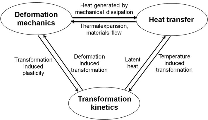 | Figure 1. Interactions between the three main physical phenomena in materials processing |
The physical phenomena involved in metal processing as well as their interactions and interdependencies are shown in Fig. 1. An accurate coupling of these phenomena is essential to achieve reliable simulation. The mathematical treatment of heat transfer (temperature field calculation) and deformation mechanics (stress-strain field computation) are usually dealt with in CAE simulation packages. Nonetheless, their governing equations are described below. CAE packages do not have the capacity of calculating transformation kinetics. Instead they rely on external user inputs typically in the form of TTT or CCT diagrams, the modelling of which is given in Session 3.
2.1. Heat Transfer
The temperature field is governed by the following equation:[3]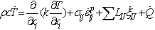 | (1) |
where ρ, c, k and LIJ are density, specific heat, thermal conductivity and latent heat from phase I to phase J, produced by the progressive Jth constituent with volume fraction ξIJ, respectively. Q is the heat generated by external heat sources. is the time differentiation of ξIJ and is termed the transformation rate. The 1st term on the right hand side is from Fourier’s law of heat conduction. The 2nd, 3rd, and 4th terms represent the heat due to plastic deformation, the heat absorbed or released during phase transformation, and other heat sources.
2.2. Deformation Mechanics
The (tensor of) total strain generated during processing can be decomposed into various individual strain contributions as follows, given in the form of strain rate for ready adaptation in CAE analysis:[4]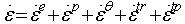 | (2) |
where εe, εp, εθ, εtr, and εtp are the elastic, plastic, thermal, phase transformation, and transformation plasticity strain contributions, respectively. The calculation of εtr and εtp is described below.Transformations from austenite to ferrite, pearlite, bainite and martensite give rise to additional strain. This additional strain is one of main factors causing local deformation of the steel part and is proportional to the relative difference in the volume fraction of each phase transformed as follows: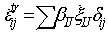 | (3) |
where βIJ is transformation expansion coefficient and it assumes that all of the phase I transforms to phase J instantaneously, and δij represents the Kronecker delta.Transformation plasticity is a deformation that appears in a transforming material under an applied stress even for the stresses lower than the yield stress of the phases.[5] It will be presented in the directions of the deviatoric stress components. The transformation plasticity strain in rate term during transformation from phase I to phase J is expressed as:[4,5]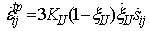 | (4) |
where KIJ and sij represent the transformation plasticity coefficient and the deviatoric stress, respectively.
3. Modelling of Materials Properties
Simulation of heat transfer requires the knowledge of thermal conductivity and heat capacity, and deformation simulation requires elastic modulus, Poisson’s ratio, thermal expansion coefficient, strength and flow stress curves. All of these properties are required as a function of temperature and/or strain rate. Phase transformation simulation requires the knowledge of transformation kinetics, as well as heat evolution and volume change during transformations. This session briefly introduces the material models developed to generate the above property data. An alloy used in later case studies is AISI 4140 (composition in wt%:Fe-0.40C-0.20Si-0.85Mn-0.95Cr-0.20Mo), so the example calculations shown in this session are for this alloy.
4. TTT/CCT Diagrams
Significant work has been undertaken to develop material models that can calculate TTT and CCT diagrams for steels, and now such calculation can be performed for a wide range of steels, including medium to high alloy types, tool steels and stainless steels.[6] The present model for the transformation from austenite to ferrite, pearlite and bainite is based on a previous model proposed by Kirkaldy et al.,[7] and it takes on the following form, which calculates the time (τ) to transform x fraction of austenite at a temperature T,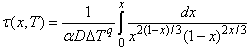 | (5) |
where α=β2(G-1)/2, β is an empirical coefficient, G is the ASTM grain size, D is an effective diffusion coefficient, ΔT is the undercooling, and q is an exponent dependent on the diffusion mechanism. Once the TTT diagram is calculated, the CCT diagram can be obtained using well-established additivity rules.[7]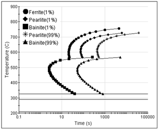 | Figure 2. Calculated TTT diagram of steel 4140 |
An accurate description of the martensitic transformation is of great importance because of the large volume change associated with this transformation. The amount of martensite, fM, as a function of the undercooling ΔT below martensite start temperature Ms is calculated using the following equation: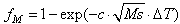 | (6) |
The calculated TTT diagram of AISI 4140 steel is shown in Fig. 2, based on austenite grain size ASTM 9 and austenisation temperature 900°C.
4.1. Physical/thermophysical Properties
JMatPro’s ability to calculate physical and thermophysical properties has been well documented in previous work for various metallic systems[8]. The calculation basically consists of three steps. Firstly, the microstructure iscalculated based on thermodynamics and phase transformation kinetics, which gives the amount and constituent of each phase in the alloy. Secondly, for each individual phase, its property is calculated based on its constituent known from the first step. Once the property of each individual phase is defined, finally, the property of the alloy can be calculated via appropriate mixture models.[9,10] The properties that can be modelled include density, molar volume, thermal expansion coefficient, thermal conductivity, Young’s modulus, Poisson’s ratio, specific heat, and latent heat. Naturally such material properties can be provided for each phase when needed.Heat treatments consist of heating and cooling and it is important to know the materials properties in such cycles. The linear expansion of alloy 4140 during a thermal cycle is shown in Fig. 3, where both heating rate and cooling rate are set as 10°C/s. 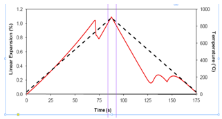 | Figure 3. Linear expansion of alloy 4140 during a heating and cooling cycle, both at 10°C/s |
4.2. Mechanical Properties
The calculation of strength/hardness of an alloy during cooling has been described previously.[11,12] JMatPro is capable of providing the strength of either the overall microstructure or that of each phase. Fig. 4 is the calculated σ0.2 proof stress as a function of temperature for each phase in AISI 4140 during cooling at 10°C/s.The approach for the calculation of flow stress models has been described in Ref.13. The flow stress curves at a fixed strain rate of 1.0 s-1 of the austenite phase at various temperatures is shown in Fig. 5, and it can be seen the model calculates three types of curves: work-hardening only (e.g. 600°C), a mixture of work-hardening and flw softening (e.g. 700°C and 800°C), and flow softwening only (e.g. 900°C).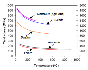 | Figure 4. Proof stress of various phases during cooling at 10°C/s |
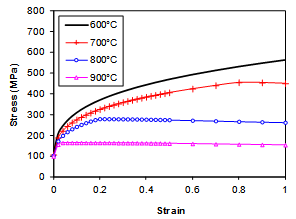 | Figure 5. Flow stress curves of austenite at various temperatures, strain rate 1.0 s-1 |
5. Case Studies – Linking JMatPro with CAE Packages for Process Simulation
The material data calculated using JMatPro have been used as inputs to a number of CAE packages for the simulation of casting,[14,15,16] heat treatments,[17,18] and forming.[19] Two case studies are provided here to highlight this application.
5.1. Prediction of Quench Distortion
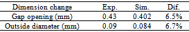
The standard Navy C-ring test is used in this work to evaluate quench distortion of an AISI 4140 steel. The C-ring was first heated to 900°C in a furnace and held for 1 hour, followed by oil quenching. The calculated material data have been used as inputs to DEFORMTM-HT[20] to carry out the heat treatment simulation, and and details of this study can be found in Ref.18.Fig. 6 shows the simulated martensite distribution on the C-ring surface at different stages of quenching, as well as the dimensional displacement. The specimen was initially expanded when heated to become fully austenitised. After 4 seconds into quenching, martensite starts to form in the region close to the C-ring gap. After 10 seconds, practically all the thermal expansion disappears, but martensite formation is still in progress, which is responsible for the further distortion. As can be seen from the microstructure after 25 seconds of cooling that the martensite formation in the thicker portion of the C-ring is associated with the final opening of the ring gap and the outside diameter of the ring. A comparison between the experimental and predicted values for the gap opening and the outside diameter was given in Table 1. It can be seen that the relative difference for gap opening and outside diameter increase are both smaller thn 7%.Table 1. Comparison between experimental (Exp.) and simulated (Sim.) results
 |
| |
|
5.2. Simulation of Hot Stamping
The hot stamping operation investigated in this work is a V-bending process of an alloy 22MnB5:Fe-0.24C-0.17Cr-1.14Mn-0.27Si-0.036Ti-0.003B in wt%. The CAE package used here is DEFORMTM-HT, and details of this study can be found in Ref.19.The temperature field, cooling rate at each position and volume fraction of martensite formed in the part are shown in Fig. 7, respectively. It corresponds to 1.6 seconds into quenching, i.e. the onset of martensite formation. Fig. 8 compares the experimental springback effect with simulation. The die angle is 60°. In experiment, the final angle changed from 60° to 61.5° due to springback, whereas that change in simulation is from 60° to 62°.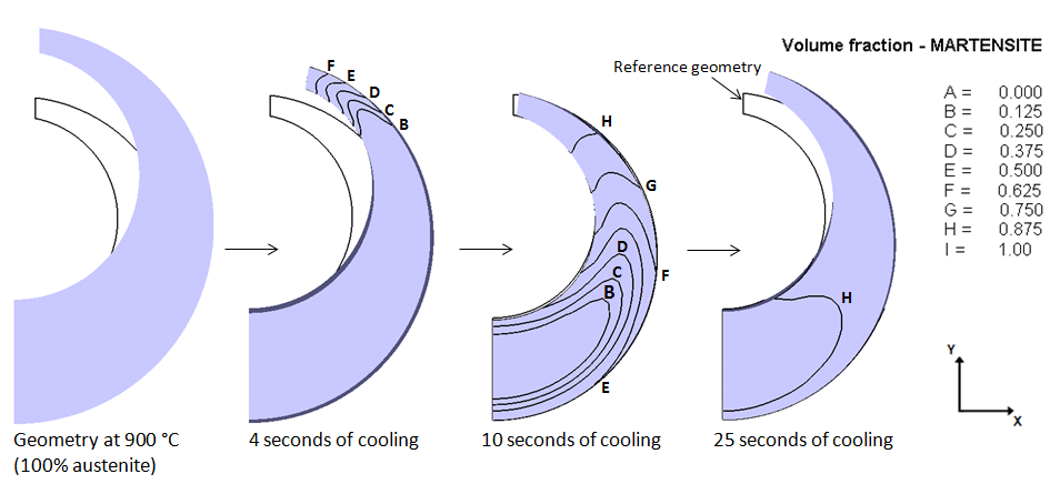 | Figure 6. Martensite formation on the C-ring during the cooling simulation |
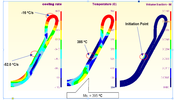 | Figure 7. Temperature field, cooling rate distribution and onset of martensite formation (about 1.6 seconds into quenching) |
6. Summary
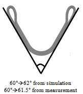 | Figure 8. Comparison of experimental and simulated final shape |
Reliable simulation of metal processing requires accurate material data, the lack of which has been a common problem, even though there are many simulation packages available. The success in the development of computer software JMatPro for material property modelling has provided a viable solution to this problem and now most of the data required by processing simulation can be calculated. The calculated property data have been used as direct inputs to CAE simulation packages to perform forming and heat treatment simulation software. This has significantly reduced the amount of experimental work required before any simulation attempts, and is a big step forward towards true virtual design and simulation.
References
| [1] | http://www.sentesoftware.co.uk, Sente Software Ltd., U.K. 2012. |
| [2] | Z. Guo, N. Saunders, A.P. Miodownik, J.P. Schillé: Mater. Sci. Eng. A, 2009, 499: 7-13. |
| [3] | K. Arimoto et al.: SFTC Paper #347, Scientific Forming Technologies Co. |
| [4] | K. Arimoto et al.: SFTC Paper #370, Scientific Forming Technologies Co. |
| [5] | S. Denis, E. Gautier, A. Simon, G. Beck: Mater. Sci. Technol., 1 (1985) 805-814. |
| [6] | N. Saunders, Z. Guo, X. Li, A.P. Miodownik, J.P. Schillé: The calculation of TTT and CCT diagrams for general steels, Internal report, Sente Software Ltd., U.K., 2004. |
| [7] | J.S. Kirkaldy, D.Venugopolan, in: Phase transformations in ferrous alloys, eds. A.R. Marder and J.I. Goldstein, AIME, (Warrendale, PA: AIME, 1984) 125. |
| [8] | Z. Guo, N. Saunders, A.P. Miodownik, J.P. Schillé: Mater. Sci. Eng. A, 413-414 (2005) 465-469. |
| [9] | Z. Fan, P. Tsakiropoulos, A.P. Miodownik, J. Mat. Sci., 29 (1994) 141. |
| [10] | A.P. Miodownik, N. Saunders and J.P. Schillé, unpublished research. |
| [11] | Z. Guo, N. Saunders, A.P. Miodownik, J.P. Schillé, in: The 2nd International Conference on Heat Treatment and Surface Engineering in Automotive Applications, 20-22 June, 2005, Riva del Garda, Italy. |
| [12] | Z. Guo, N. Saunders, A.P. Miodownik, J.P. Schillé: International Journal of Microstructure and Materials Properties, 4 (2009) 187-195. |
| [13] | Z. Guo, N. Saunders, J.P. Schillé, A.P. Miodownik, in: MRS International Materials Research Conference, 9-12 June, 2008, Chongqing, China. |
| [14] | K.D. Carlson, S. Ou, C. Bechermann, Metall. Mater. Trans. B, 2005, 36B: 843-856. |
| [15] | X. Zhang et al., Israel Journal of Chemistry, 2008, 47 (3-4): 363-368 |
| [16] | Z. Guo, N. Saunders, E. Hepp and J.P. Schillé, Modelling of material properties - A viable solution to the lack of material data in casting simulation, in: The 5th Decennial International Conference on Solidification Processing, 23-25 July, 2007, Sheffield, U.K. |
| [17] | J. Fu et al., Advanced Materials Research, 2011, 317-319: 19. |
| [18] | A.D. da Silva et al., Distortion in Quenching an AISI 4140 steel C-Ring – Predictions and Experiments. Accepted for publication in Materials & Design, 2012. |
| [19] | Z. Guo, G. Kang, N. Saunders, Modelling of materials properties used for simulation of hot stamping, in: The 13th International Conference on Metal Forming, 19-22 September 2010, Toyohashi, Japan |
| [20] | DEFORMTM-HT version 10.1, Scientific Forming Technology Corporation, Columbus, Ohio, USA. |
 Abstract
 Reference
 Full-Text PDF
 Full-text HTML