Rongshan Qin1, Xu Tan2
1Department of Materials, Imperial College London, London, SW7 2AZ, United Kingdom
2Graduate Institute of Ferrous Technology, Pohang, 790-784, Republic of Korea
Correspondence to: Rongshan Qin, Department of Materials, Imperial College London, London, SW7 2AZ, United Kingdom.
| Email: |  |
Copyright © 2012 Scientific & Academic Publishing. All Rights Reserved.
Abstract
A scheme has been developed to integrate the phase-field model with the homogeneous deformation. This has been applied to the simulation of the microstructure evolution during warm rolling of steels. The phase transition is characterized by the evolution of a phase-field order parameter. The rolling of the steels is calculated by the displacement of vectors in materials by the deformation matrix. The governing equation for phase-field order parameter is solved numerically in the irregular and changing lattices. Significant discrepancies of crystal morphologies are observed in crystal growth before deformation, deformation of materials after crystal growth and deformation of materials while crytal growing. Those three thermomechanical processing conditions can be considerred as the cases of hot rolling, cold rolling and warm rolling, respectively. It has been found that the interface anisotropy plays an important role for the observed microstructural descrepacies. Other mechanisms affecting the grain morphologies are discussed for various thermomechanical processing of steels.
Keywords:
Steel, Warm Rolling, Phase-Field, Homogeneous Deformation, Microstructure
Cite this paper: Rongshan Qin, Xu Tan, Phase-Field Simulation of the Thermomechanical Processing of Steels, International Journal of Metallurgical Engineering, Vol. 2 No. 1, 2013, pp. 35-39. doi: 10.5923/j.ijmee.20130201.05.
1. Introduction
Thermomechanical processing implements heat and stress in tailoring the microstructure of steels. Hot rolling, cold rolling and warm rolling are characterized by the sequences of austenite-ferrite phase transformations regarding to the mechanical deformation, i.e., the hot rolling deforms steels before austenite-ferrite phase transition, cold rolling deforms steels after this phase transition, and warming rolling deforms steels during the phase transition. In practice, steel processing may use more than one rolling scheme, e.g. starting from the hot rolling but completing at the warm rolling temperature. Warm rolling has attracted significant attention due to its complexity. Experimental observations such as the evolution of microstructure[1] and texture[2] in warm rolling of low carbon steels have been reported. Numerical simulations including finite element calculation are carried out to the investigation of the warm rolling[3-4]. This work aims to study the microstructure evolution in warm rolling by coupling the phase-field model with homogeneous deformation theory.The deformation of materials can be described by either the equal-stress or equal-strain approximations. The homogeneous deformation is an equal-strain method, and is suitable particularly for those deformations without the formation of cracks and other defects. The fundamental principle of this method is represented by following equation | (1) |
where S is called the deformation matrix.  and
and  are the vectors before and after the deformation, respectively. The elements of the matrix S take different values to represent various types of homogeneous deformations. Zhu et al has applied the homogeneous deformation method to the study of the metallography of a tetrakaidecahedron grain[5]. Chae et al applied the method to the deformation of non-uniform grains[6]. The computation of the microstructure evolution in mechanical deformation can be achieved by applying Eq. (1) to every pixel of the micrograph images.The microstructure evolution in phase transition, including both displacive transformation and reconstructive transformation, can be calculated in the framework of a phase-field model[7]. The model introduces an order parameter (
 ) to represent the physical state of the materials.
  takes one value from one phase to another value in another phase and changes smoothly from one value to another across the interface. The governing equation for the phase-field order parameter can be derived explicitly from the second law of the thermodynamics. The parameters in the governing equation can be obtained by manipulating the governing equation to the simplest conditions. For a case where the phase transition is driven by a constant driving force and the solute and temperature heterogeneous are ignored completely, the governing equation for the phase-field order parameter is[8]
 | (2) |
where  is called the phase-field mobility related to the interface kinetics. εis called the gradient energy coefficient reflected the interface energy and the interface anisotropy.
  is the free energy density of the material and is a double well potential in non-equilibrium state. The calculation of the phase transition is achieved by solving Eq. (2) with time iteration. Application of the phase-field models in various materials have been summarized in a number of review articles, as listed in ref.[9].In the present work, the phase-field model has been coupled with the homogeneous deformation theory. Application of the coupled model to the thermomechanical processing of steels has been demonstrated. The microstructural evolution in various processing conditions is calculated. The mechanisms responsible for the characterized microstructures will be investigated.
2. Theoretical Consideration
Warm rolling has two coupled physical processes, namely the phase transition and materials deformation. Phase-field model can be used to address the microstructure evolution in phase transition. Homogeneous deformation is to be used to address the mechanical deformation. Warm rolling is taking place in relative high temperature. This enables the ignorance of the residual stress in materials which otherwise will affect the free energy density and interface energy. The formation of various defects such as dislocations, voids and cracks are ignored. It is also assumed that the time of each rolling pass is short enough in comparison with the overall phase transition time. This is reasonable because the phase transition takes place in a wide temperature range but the temperature dropping during each rolling pass is small. With such consideration, we can ignore the phase transition during the rolling pass, i.e., phase transition takes place in many time steps but each rolling pass can complete within a single time step.The double well potential for the free energy density can be represented as where
where  . ω is related to the barrier height and can be determined by the interface thickness (2λ) and interface energy (σ) via.
 and
and  are the free energy density of bulk phases represented by
  and
and  , respectively.
  is associated with the volume fraction of the phases. This gives the second term in the right-hand-side of Eq. (2) as
 | (3) |
where  .
.  is the driving force for phase transition. The gradient energy coefficient ε in Eq. (2) is related to the interface energy and its anisotropy. For cubic crystal, the anisotropic interface energy can be represented as[8]
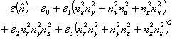 | (4) |
where  is the normal vector to interface and is determined in phase-field calculation
  by. The coefficients
  ,
,  ,
,  and
and  are determined by
  | (5.1) |
 | (5.2) |
 | (5.3) |
 | (5.4) |
The coefficients  ,
,  ,
,  and
and  are determined according to the interface anisotropy. A method to specify those coefficients for various metals was presented in our earlier works[8, 10].In phase transition, Eq. (2) is calculated in space represented by discrete lattices that can be arranged as regular or irregular patterns. Crystal growth is obtained by iteration of Eq. (2) in a series discrete time steps. Each rolling pass is calculated within one time step according to Eq. (1) and the calculation is performed throughout the discrete lattices in space. The different values of
  is plotted with different colours so that the crystal morphology can be examined.
3. Numerical Calculation
The materials are initially represented by rectangular lattices with lattice distance in all three dimensions equivalent to Δh. The finite difference method gives the first order differentiation of phase field order parameter regarding to the space coordinate parameters as following forward step approximation | (6) |
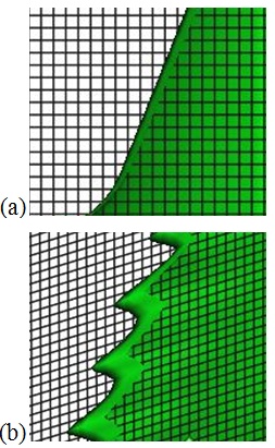
where the meaning of  is illustrated in Fig. 1(a). After the shape deformation, the rectangular lattices are not able to retain its original shape in all three dimensions. In some cases, the lattices are arranged in a shape similar to that illustrated in Fig. 1(b). The partial difference regarding to space coordinate should use more generic equation of followings[11]
 | (7) |
In discrete format as that illustrated in Fig. 1(b), it has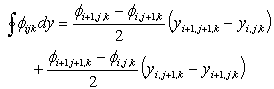 | (8) |
To reduce the mathematical error, following calculation is applied in the calculation | (9) |
 | Figure 1. Schematic diagrams of (a) rectangular and (b) non-rectangular lattices |
The important condition for using Eq. (8) and Eq. (9) is that all the four lattice points should be in the same plane. The differentiation regarding to time is represented by following explicit discrete approximation in a time step of Δt | (10) |
In the present simulation, a rectangular lattices of 160×160 ×120 are defined initially. The initial condition for the phase field order parameter is specified according to following conditions The constant driving force is selected as
  . The experimental measurement gives the average interface energy between face centred cubic and body centred cubic crystals of steel as k0= 0.8 J/m2. Because the actual anisotropic property between austenite and ferrite phases is not known, one uses a general expression of the anisotropic interface energy for the cubic metals and chooses following arbitrary values for the calculation:
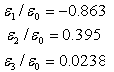 | (11) |
The corresponding anisotropic interface energy in its polar diagram is illustrated in Fig. 2. Other parameters include M=100 and λ=14.3 nm. This gives ω=1.3510-9 m3/J and ε0=2.48810-4  . Without consideration of deformation, the crystal morphology at t = 12000 time steps is demonstrated in Fig. 3. This is a typical anisotropic crystal. Due to the assumption of constant driving force and ignorance of heat and mass transfer and also the ignorance of fluctuation, there is no equilibrium shape of the crystal can be obtained.
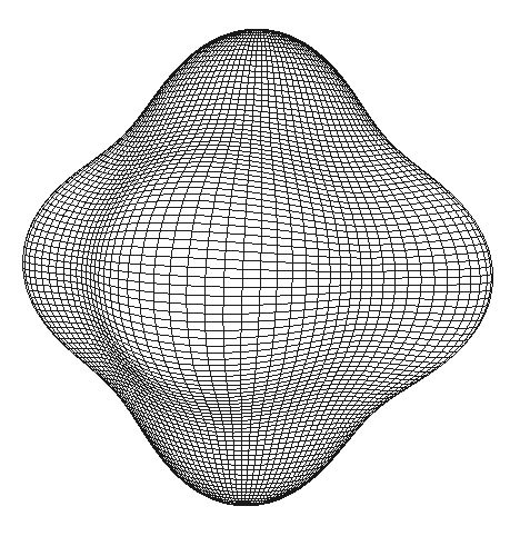 | Figure 2. Polar diagram of anisotropic interface energy represented by Eq. (4) with coefficients value in Eq. (11)[12] |
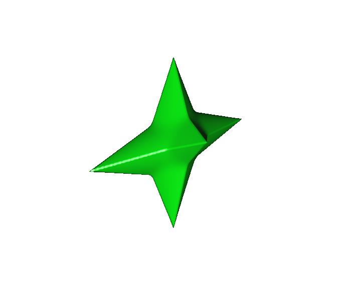
Application of shear deformation to the crystal once after 12000 steps of crystal growth gives the crystal morphology demonstrated in Fig. 4. The deformation matrix for shear deformation is After one rolling at the 12000 time steps, the morphology of crystal changes into that demonstrated in Fig. 4. The topological geometry of the crystal is not changed but the morphology is homogeneously sheared alone z-direction.
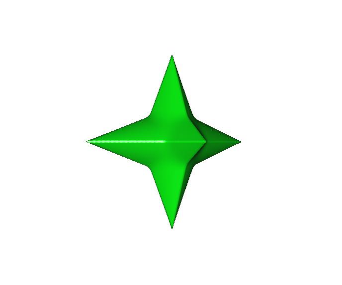 | Figure 3. The crystal morphology without deformation at 12000 time steps |
 | Figure 4. The crystal morphology after the shear deformation at 12000 time steps |
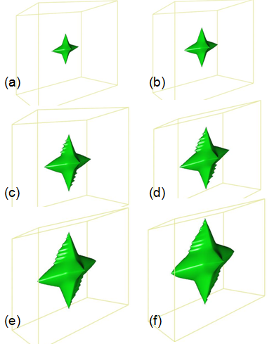 | Figure 5. Crystal shape at (a) 6000, (b) 8000, (c) 10000, (d) 12000, (e) 14000 and (f) 16000 time steps. The shear deformation applied after every 6000 time steps |
Another case is to have the shear deformation after every 6000 time steps of crystal growth. The crystal morphological evolutions are demonstrated in Fig. 5. It can be that the crystal morphology is completely different from that of Fig. 3 and Fig. 4.In summary, Fig. 3 corresponding a crystal growth without deformation. This is similar to the microstructure evolution in hot rolling. Fig. 4 corresponding to a mechanical deformation after crystal growth. This is similar to the case of cold rolling. Fig. 5 gives microstructure evolution with phase-transition and mechanical deformation taking place in a same period, and is corresponding to warm rolling. Warm rolling generates significant different microstructure in comparison with hot rolling and cold rolling.
4. Discussion
 | Figure 6. Lattices and crystal interfaces after shear deformation and crystal growth |
It can be seen from Fig. 5 that the major difference of the crystal morphology is at the crystal arms facing and parallel to the shear direction. The interface at this direction is getting more steeper after shear deformation. This makes its interface energy bigger than before deformation. To reduce the interface energy, crystal growth along this direction is accelerated so that there are less amount of interface will be faced to this direction and hence the total surface energy and total free energy of the system can be reduced. This can be clearly seen in Fig. 6. The same situation appears to the interfaces at the plane diagonal direction. It can be seen that the similar crystal morphology evolution are appeared in that crystal arm. On the contradictory, the interface parallel and along the shear direction is getting less steep and more close to an interface normal direction which possesses smaller interface energy. The crystal growth at those areas is not encouraged in order to maintain its smallest interface energy and hence the total free energy. This is clearly seen in Fig. 5. The shear deformation does not change the orientation of other four crystal arms significantly. Therefore, the crystal morphology at those places are not altered obviously.In summary, the combination of deformation and interface anisotropy are the major reason to cause the unusual microstructure evolution. Quantitative and more general description of this effect requires more systematic investigations.
5. Conclusions
A phase-field model has been coupled to the homogeneous deformation method. The integrated scheme is able to simulate the thermomechanical processing of steels. The microstructure evolution due to phase transition can be handled by the phase-field model. The microstructure evolution due to mechanical deformation can be calculated by the deformation theory. The coupled scheme has been applied to the crystal growth in warm rolling. The drastic microstructure alteration in this case is considered due to the deformation of the interface and the anisotropic properties of the interface.
ACKNOWLEDGEMENTS
RQ is grateful to Professor HKDH Bhadeshia from University of Cambridge for invaluable discussion and to TATA Steel and the Royal Academy of Engineering for financial support of this work.
References
| [1] | G. H. Akbari, C.M. Sellars and J.A. Whiteman, Acta Mater, Vol. 45, No. 12, 1997, p. 5047. |
| [2] | A. Haldar and R.K. Ray, Mater. Sci. Eng. A, Vol. 391, No. 1-2, 2005, p. 402. |
| [3] | J. Majta and A.K. Zurek, Int. J. Plasticity, Vol. 19, No. 5, 2003, p. 707. |
| [4] | C.A. Greene and S. Ankem, Mater. Sci. Eng. A, Vol. 202, No. 1-2, 1995, p. 103. |
| [5] | Q. Zhu, C.M. Sellars and H.K.D.H. Bhadeshia, Mater. Sci. Tech., Vol. 23, No. 7, 2007, p. 757. |
| [6] | J.Y. Chae, R.S. Qin and H.K.D.H. Bhadeshia, ISIJ international, Vol. 49, No. 1, 2009, p.115. |
| [7] | R.S. Qin and H.K.D.H. Bhadeshia, Mater. Sci. Tech., Vol. 26, No. 7, 2010, p.803. |
| [8] | R.S. Qin and H.K.D.H. Bhadeshia, Acta Mater., Vol. 57, No. 7, 2009, p. 2210. |
| [9] | R.S. Qin and H.K.D.H. Bhadeshia, Curr. Opin. Solid State Mater. Sci. Vol. 15, No.3, 2011, p.81. |
| [10] | R.S. Qin and H.K.D.H. Bhadeshia, Acta Mater., Vol. 57, No. 11, 2009, p.3382. |
| [11] | M. Shashkov and S. Steinberg, Conservative Finite-Difference Methods on General Grids, 1st Edn., CRC Press, 1996, pp. 26-45. |
| [12] | R.S. Qin, Mater. Manufac. Proc., Vol. 26, No. 1, 2011, p. 132. |
 Abstract
 Reference
 Full-Text PDF
 Full-text HTML