1. Introduction

Fine-scale spatial genetic structure (FSGS) can be defined as the non-random spatial distribution of genotypes in a population. It is a key characteristic of many plant populations ([25],[59],[76]). This was first conceived at the broader scales as ‘isolation-by-distance’ which could result solely from progressive limits to dispersal ([46],[78]). Later, since true Panmixia was found not to occur at most large landscape scales, the ‘stepping stone’ model was proposed in which these large areas were broken down into smaller pockets of breeding individuals characterized by a smaller N_e (effective neighbourhood size) ([6],[37],[66],[67]). At still ‘higher’ spatial resolutions within continuously distributed plant populations, gene flow by near neighbour pollen ([29],[77]) coupled with the successful establishment of these seeds/seedlings was proposed to lead to localized ‘hotspots’ of genetic consanguinity ([43],[48],[68]). In sedentary higher plants, as distinct from animals in which individuals can migrate on short temporal scales, FSGS, broad and fine scale, is predominantly determined by the dispersed amounts and distances (axial variance) of pollen and seed ([18],[26]). Leptokurtic distributional patterns of pollen and seed are well known in plants[40].

It has been suggested that core, stable populations of long-lived shrubs and trees are less likely to exhibit FSGS, although there are exceptions, especially in populations that are on the edge of the species’ distributional range[52]. Lowbush blueberry (VacciniumangustifoliumAit.) is a woody shrub in that it is long lived and has a clonal habit and as such it was not known whether it is characterized by FSGS. This fruit-producing shrub also is unique as an agricultural crop because fields are wild managed patches instead of sown cultivated fields and the genetic population structure of managed patches does not differ from natural habitat areas (Drummond, unpublished data). Natural colonization and dispersal processes over 13,000 years, since the retreat of the Laurentide ice-sheet alongcoastal Maine, are presumed to have produced the highly variable distributions in lowbush blueberry fieldstoday[11] . Being sedentary flowering plants, the FSGS of blueberryfields would result entirely from the combined effects of fitness and dispersal distances of pollen and seed[26].

In recent years, molecular approaches have begun to be used for estimating genetic relationships among genotypes of wild, lowbush blueberry. Of particular interest is the use of molecular markers to assess relationships among individual genotypes (clones) which are proximally situated within fields because they are likely to be intensive pollen exchangers, according to near-neighbour bee pollination models ([7],[8],[12],[49]) and observed pollination in response to bee foraging ([5],[22]).

Lowbush blueberry is tetraploid (2n=4x=48), highly polymorphic, primarily outcrossing, and taxonomically complex ([30],[31],[75]). The development and use of molecular markers, including RAPDs, EST-PCR (Expressed Sequence Tag- Polymerase Chain Reaction) and SSRs (which are increasingly being gleaned from the growing EST libraries of highbush blueberry,V. corymbosum L.) ([3],[10],[12],[57],[58]), have stimulated many recent investigations of the genetic structure of lowbush blueberry populations. Within-field level FSGS is highly germane since lowbush blueberry has long been documented as predominantly self-infertile (outcrossing) because of early-acting, inbreeding depression[33]. Based on the relative self-infertility and high extant genetic loads within lowbush populations, a leading conjecture has been that pockets of highly related clones might be a cause of dramatic yield variation among clones within the same field ([33],[49],[50]).

Using EST-PCR markers,[9] made the first attempt at characterizing SGS at several spatial scales in lowbush blueberry: 1) within-clones, 2) among-clones within-fields, and 3) among four spatially distinct fields. Only a slight trend (p< 0.10) of within-field positive FSGS could be found in two fields, despite the fact that individual clones appeared to be genetically homogeneous. However, strong among-field variation was found at longer distances (~ 65 km). Due to the scope of this multi-year study and its primary focus on inter-clone yield variation, sample sizes were somewhat constrained (7 – 24 clones per field), thus we had reduced statistical power for detecting FSGS. Even so, a few pairs of neighbouring clones (22%) appeared to be significantly related using a non-parametric, 2-dimensional local spatial autocorrelation analysis (2D-LSA)[55]. Despite this, the more general view suggested that clones within fields appeared to be predominantly non-structured.

This paper represents a second more experimentally rigorous attempt at characterizing within-field FSGS using larger sample sizes, a smaller range of between-clone distances, and a higher resolution DNA marker methodology. Here, two different spatial collection designs were employed: 1) a contiguous design in which we sampled and analysed every clone within a 0.35 ha area, and 2) a more biologically conceived design in which we sampled two high and two low-yielding clones from each of two fields along with five clones immediately surrounding each of these focal eight plants. In conjunction, both the contiguous andneighbourhood designs focused on maximizing sampling intensity as well as implementing a more efficient sampling design as compared to those used in the study of[9]. In addition to the inherent benefits of increasing sampling intensity, we decreased the distance between sampled genotypes in the contiguous design by sampling every plant or clone within a designated area[4]. In the neighbourhood design, we sampled the complete surrounding neighbourhood of possible adjacent (touching)clones around a focal recipient plant, not exclusivelypairs of plants as in the previous study.

2. Materials and Methods

2.1. Study Sites and Sampling

Plant materials for both designs (contiguous and neighbourhood) were collected in June and August, 2009, from two managed lowbush blueberry fields in Maine. The sites are designated as the Blueberry Hill Research Farm (B: 44°38’ N, 67°38’ E) and Columbia (C: 44°40’N, 67°52’ E) and are 19 km apart, near Jonesboro, ME.

2.2. Contiguous Design Experiment

Samples for the contiguous design were collected at the Columbia field site. A sampling protocol was conducted using a design of an expanding spiral starting from a randomly picked centre clone. Since a total of 95 clones could be evaluated together on one 96-well plate (with one well for a molecular ladder), every clone in this spiral transect was sampled until a total of 95 clones was reached. One clone’s DNA did not amplify well leaving a total of n=94 for this study. These 94 clones occupied an area of 0.35 ha.

2.3. Neighbourhood Design Experiment

In order to look for possible associations between FSGS and yield in future studies, we chose two high and two low producing clones (as measured by open pollination fruit set from the previous yield year) from both the Blueberry Hill and Columbia sites. These clones served as the central bearing females of each neighbourhood. We defined a neighbourhood as a localized pocket of likely pollen exchangers consisting of a centrally located clone surrounded by five adjacent likely pollen donors as inferred by bee foraging patterns. Four neighbourhoods of six clones (1 central female, 5 touching donors) in each of the two fields yielded a total of 48 possible clones for this study. Two pollen donors’ DNAs, BH2 (Blueberry Hill; 2^nd highest yielder) and BL1 (Blueberry Hill; 1^st lowest yielder), did not reliably amplify and had to be discarded from the study leaving these two neighbourhoods with four surrounding donors each, or 46 clones total.

2.4. DNA Extraction And EST-PCR Analysis

For both experiments, approximately 3-5 g of fresh leaf tissue was collected from the centres of all clones. Leaf samples were sent overnight on ice to the USDA/ARS facility in Beltsville, MD, USA, and there stored at -80° C until genomic DNA could be extracted. The same protocols previously described were followed for genomic DNA extraction and PCR amplification ([7],[57]). EST-PCR primers were chosen from past performance in our previous work in lowbush blueberry based on their polymorphic information content and dependability in PCR amplification. As in our previous study, bands were scored and analysed in binary fashion as dominant markers, i.e. bands present (1), or bands absent (0). However, a key difference was the change from “agarose gel electrophoresis” to a 96-well PCR format using the AdvanCE™ FS96 (Advanced Analytical Technologies, Inc., Ames, IA, USA) “capillary gel electrophoresis” system. All separations were run using the AdvanCE™ FS96 dsDNA Wide Range 50-2,000 bp (DNF-910) gel system, which was the appropriate gel system for the size of the DNA fragments we intended to score. Digital electropherogram traces were collected by monitoring the relative fluorescence intensity (RFU) as a function of migration time during separation. Band sizes were calculated from a calibration function based on a best-fit 4^th order polynomial generated from the relative migration times of the molecular weight ladder bands as derived by the manufacturer’s supplied PRO Size™ software.

2.5. Automated Scoring

Proprietary PRO Size™ software, which is included in the AdvanCE™ FS96 system, was used initially to visually select strong, clear polymorphic bands for scoring. Due to the high sensitivity and separation ability of the AdvanCE™ FS96 system in the 50-1,000 bp range, we focused on scoring markers within this range. An upper and a lower marker of 35 and 2,000 bp was used for all runs, as well as a GeneRuler™ 100 bp Plus DNA ladder (100 – 3,000 bp) (Fermentas International, Inc., Glen Burnie, Maryland, USA). Selected bands were then entered into the automated scoring module using a tolerance of + 2.5% of the band size, thus adjusting for a higher separation resolution of smaller sized fragments. For each design the results of each primer/genotype set were amalgamated into one binary matrix of 1’s and 0’s. This genetic matrix, along with the inter-clone physical distance matrix, provided the entire basic input for all downstream population genetic analyses.

2.6. Data Analysis and Statistical Methodology

We used the same distance-based methods for our population genetic analyses as in[8]. For each experimental design, contiguous and neighbourhood, a pairwise, symmetric, individual-by-individual (N x N) genetic distance matrix was calculated after[35] using the current GenAlex v. 6.41[55]. With dominant markers, these pairwise distances are equivalent to the number of band differences between each pair of genotypes. Using GPS coordinates for each sampled clone, a geographic distance matrix was also constructed, which is a symmetric matrix consisting of distances in meters between all pairs of genotypes. For example, in the contiguous study, which used 94 genotypes (clones), this resulted in 4,371[(94 x 93)/2] pairwise distances for both matrices. These two distance matrices, genetic and geographic, were used in all analyses including Analyses of Molecular Variance (AMOVA; Φpt), Spatial Autocorrelation (SA) testing via the construction of correlograms, and 2-dimensional local spatialautocorrelation (2D-LSA ) ([14],[28],[55],[61],[62]). A more liberalized value of p = 0.10 was used for the 2D-LSA tests in an ‘explorative’ manner[68]. For all non-parametric tests of significance including AMOVA, SA, and 2D-LSA, permutations and/or bootstraps were used (n=9,999). NTSYS v. 2.2 was also used to estimate a ‘goodness of fit’ of clustering ([56],[65]), referred to as the cophenetic correlation[56] which is a linear correlation between the distance matrix and the cophenetic matrix (the minimum merging distances of clusters,[36]).

For the neighbourhood design we scored all 46 genotypes from both fields as a group. This allowed the construction of a nested AMOVA with fields (Blueberry Hill and Columbia) as regions or statistical blocks, and the eight neighbourhoods as populations within fields. In addition, we performed an AMOVA analysis on Blueberry Hill and Columbia separately, in order to detect possible differential apportionment of variation between the two fields.

A critical parameter in any spatial autocorrelation analysis is the choice of distance class size. In the contiguous design, for the generation of the correlogram, we based the decision on the largest distance between any two adjacent clones, which was 7.3 m. Thus, we chose multiples of 7.5 m as the distance classes because every single nearest neighbour pair would be included within the first distance class. In the 2D-LSA analysis, it is necessary to select the number of nearest neighbours to include in calculating an ‘r’ value and associated estimated P-value via non-parametric permutation methods. In this method of estimating local SA, a correlation coefficient, lr, is generated for pairs of individuals that fall within a certain distance class, which in this case is a specialized distance class constructed from all the inter-clone distances. A module is included for 2D-LSA as an alternative form of SA in GenAlEx 6.41 in which a special kind of distance class is used, namely the distance(s) between a pivotal individual and an experimentally chosen number of nearest neighbours. This non-parametric, permutation approach is similar to Moran’s – I^(h) ,except that it conditionally weights the genotypes in the distance matrix for how many times that genotype appears in that distance class[63]. The calculated correlation coefficient is a proper correlation coefficient in having a mean of ‘0’ in the absence of autocorrelation and a domain of[-1, +1]. Based on the SA correlogram analysis, the ‘r’ value reached zero, or insignificance, at approximately the 15-meter distance class. A module in GenAlEx 6.41 allows the determination of the sequence of next nearest neighbour distances from each pivotal clone in the study (n = 94). In this data set, every subset of an individual and its four nearest neighbours fell within 15 m ([21],[54],[63]); thus, this number was chosen for the bootstrap analysis to test for ‘hotspots’ of individual clones that were significantly related relative to a null distribution[68]. For the 2D-LSA analysis in the neighbourhood study, the number of nearest neighbours was five.

3. Results

3.1. Primers, Numbers of Bands, Goodness of Fit

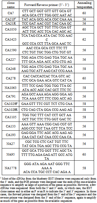
Table 1 lists the EST-PCR primers used in this study for both designs. The EST-PCR primers used were a subset of those used in our previous SGS study in lowbushblueberry[9]. For the contiguous study, 90 bands were scored from 17 primer pairs (5.3 bands per primer) with an NTSYS ‘goodness of fit’ cophenetic correlation of 0.78. For the neighbourhood study, 115 bands were scored from 13 primer pairs (8.8 bands per primer) with a ‘goodness of fit’ value of 0.81.

3.2. FSGS Global and Local: Contiguous Study

We tested first for the broader indication of global SA via Mantel tests as implemented in GenAlEx 6.41 on the 94 samples in the contiguous study. Using the untransformed geographical distance matrix shuffled against the genetic distance matrix, a non-significant result (P = 0.060, r= 0.060) was obtained. However, using transformed (ln (x+1)) geographical distance data, a significant result (P = 0.024, r = 0.075) was obtained. Even in this case, representing a non-linear distance by relatedness pattern, only a low proportion of the total variation in genetic relatedness could be explained by the geographic distance between clones (< 0.5%). This indicates that there is very little global SA across the entire data set. This test was not performed on the neighbourhood design since this ‘clustered’ sampling design is not appropriate for testing global SA due to many missing ‘middle’ physical distances, resulting in a highly leveraged analysis.

Figure 1 shows the standard SA correlogram resulting from the contiguous study. Since the focus of this study was to test for a positive local SA at the scale of adjacent clones (likely pollen exchangers) and because every clone’s single nearest neighbour fell within a 7.5 m range, multiples of 7.5 m were chosen for the distance classes for the correlogram. In fact, 153 pairs of clones fell within the first 7.5 m class and yielded a significant average correlation for the class of r = 0.067 + 0.022 (P< 0.001). The surplus of pairs, above the expected 94, is due to many clones having more than one neighbour (59 additional clones to the base 94) within the 7.5 m class. The higher distance classes yielded insignificant r-values, with the exception of a marginally significant negative SA (‘coldspot’) at the 30-meter class.

Figure 2 shows graphical results of the local 2D-LSA statistical analysis that was conducted on the 94 contiguous clones. For this analysis, the number of nearest neighbours was five. This design is more representative of field conditions than the “clone pairs-only” approach of our previously published study[9]. The number of nearest neighbours chosen was based on the fact that this distance included all inter-clone pairs that fell within 15 m of each other, i.e. the r value crossing the r = 0 axis which denotes the first non-significant distance class in Fig. 1.

The statistical testing for local SA in this kind of analysis is still problematic due to handling the accumulating error of many pairwise comparisons. Therefore, due to our biological knowledge of the system, it is presented as ‘explorative’ in nature[68]. In Figure 2, as a visual aid, we have placed ellipses enclosing the 11 apparent ‘local neighbourhoods’ denoting ‘hotspots’ or clusters of adjacent genetically similar individuals or clones. The approximate area of the largest of these eleven groups was 121.3 m² while the smallest was 18.6 m². There are seven subgroups of adjacent starred clones representing the very highest genetically similar near neighbour pairs. The value (or mean if multiple pairs) of the proportion similarity of these subgroups ranged from 0.53 – 0.72[56]. It is known from previous work using a group of clones of known pedigree and dominant markers that half-sib to full-sib genetic similar values range from 0.65 – 0.80[7].

Starred pairs (Fig. 2) are genetically similar at the P = 0.05 (conservative) value, while open circles represent a more liberal conjecture (P = 0.10).The ‘x’ symbols represent clones that do not show significant genetic consanguinity with their local neighbourhoods (P> 0.103). Solid versus dotted ellipses indicate neighbourhoods of all starred individuals versus neighbourhoods of mixed stars and open circles. The evidence shows that there are highly related clustered groups (‘hotspots’) set within a predominant majority of less related clones within this 0.35 ha contiguous area. In fact, 62 clones (66.0%), showed a random genetic spatial distribution in and around the significant clusters. It is interesting to note that the range of genetic similarity values was from 0.05 – 0.81, which demonstrates the large genetic diversity contained within this confined area of one field.

3.3. AMOVA and 2D-LSA: Neighbourhood Study

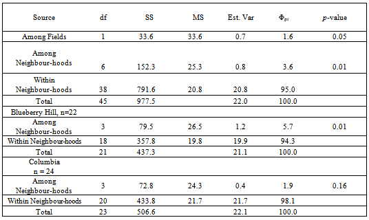
Table 2 shows the nested AMOVA results for the global neighbourhood study followed by an individual field level AMOVA for each field separately. At the highest level of variation (regional or field), a significant Φ_rtvalue of 1.6% (Among Fields/Among Fields + Total) was found (P= 0.050) indicating that Blueberry Hill and Columbia are genetically differentiated at approximately 19.0 km apart. At the next level of variation (population or neighbourhood), genetic differentiation was found with a Φ_pr value of 3.6% (P = 0.010). The value of 3.6% represents the variation among all eight neighbourhoods pooled over both fields. Further dissection using separate AMOVA’s for each field revealed that only Blueberry Hill actually showed significant genetic differentiation among neighbourhoods with a Φ_pt value of 5.7% (P = 0.011), while Columbia did not, with a Φ_pt value of 1.9% (P = 0.122).

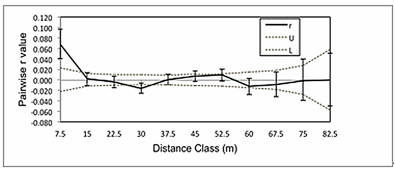Figure 1. Global spatial autocorrelation (SA) ‘correlogram’ for the contiguous design study. Pairwise genetic similarities (y-axis, r value) of clones falling within the distance class shown on the x-axis (m) are plotted against distance classes (multiples of 7.5 m). The dotted lines represent the upper and lower 95% confidence limits. Bootstrap error bars are also shown at each distance class. A significant positive SA (‘r’ centre line falling outside the 95% confidence limits) is seen in the first distance class of 7.5 m, which declines to a non-significant value at 15 m upon intersection with the x-axis. The balance of the distance classes show non-significant ‘r’ values

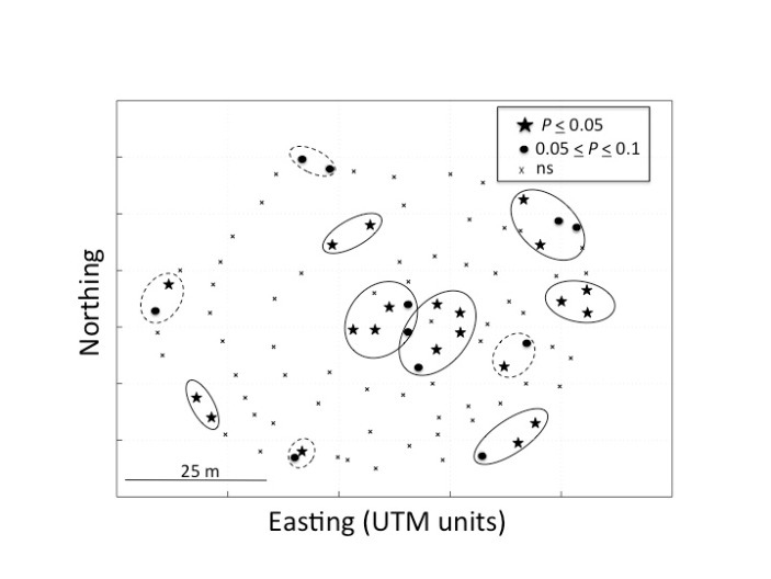Figure 2. Geographic map in Universal Trans-mercator Units (UTM) depicting locations of clones in the contiguous design study, which show related clusters (‘hotspots’) from a 2D-LSA (2- Dimensional Local Spatial Autocorrelation) analysis. The plot shows eleven clusters (ellipses containing stars and open circles), with four sub-groups of clones related at the 0.05 <P < 0.1 level and seven sub-groups of clones (at least one pair of stars) related at the P < 0.05 level. Each of the clones’ relatedness is assessed with their five spatial nearest neighbour clones and ellipses are intended as visual aids and are not quantitatively calculated

Table 3 shows the pairwise neighbourhood comparisons, Φ_ptvalues by field (below diagonal) together with their respective p-values (above diagonal). Notably, only one of the six possible pairwise Φ_ptvalues within each field was found to be statistically significant. These values of Φ_pt were 13.4% (P= 0.051) and 6.7% (P = 0.020), for Blueberry Hill and Columbia, respectively. Figure 3 shows the 2D-LSA graphical results for the neighbourhood study separately for Blueberry Hill and Columbia. The plots are standard maps of each field using Universal trans-Mercator Units (UTM) as the geographical measure of distance. The maps show the eight clusters or neighbourhoods of each field with a central ‘female’, surrounded by five touching neighbours. Starred individuals are significantly genetically similar (P < 0.10) to the other clones within their neighbourhood. The statistical significance is only relevant to the single immediate neighbourhood since five nearest neighbours to the pivotal individual were involved in the permutation test[55]. Overall, the results show a similar pattern by the clustering of hotspots against an otherwise random distribution of genotypes. The patterns shown here in Figure 3, the neighbourhood design, are similar to the patterns seen in Figure 2, the contiguous design.

Each large centre dot represents the central female of aneighbourhood with spokes connecting to the centres of the surrounding likely donors. At Blueberry Hill, two surrounding donors were omitted from the study; thus twoseparate 2D-LSA analyses were conducted using four nearest neighbours for these two neighbourhoods, and five nearest neighbours for the other two. Overall, at Blueberry Hill atotal of 5 of 22 (22.7%) pivotal clones were significantly related to the others in their neighbourhood. At Columbia, the results indicated 8 of 24 (33.3%) clones were significantly related to the others in their neighbourhood. In total,13 of 46 (28.2% compared to 34.0% in the contiguousstudy) of the clones were involved in significant withinneighbourhood relationships while the majority (71.8%), as in the contiguous study, showed a random spatial genetic pattern.

Table 1. List of the 17 EST-PCR primer pairs used throughout this study, names of EST clones from which they were derived, and annealing temperatures. EST-PCR primers were designed near the 5’ and 3’ ends of ESTs from non-acclimated (NA) and cold acclimated (CA) flower buds of highbush blueberry cultivar ‘Bluecrop’ (V. corymbosum). All of these EST-PCR primers were used in our previous FSGS study[9]. For GenBank accession numbers and BLAST results of ESTs, see the Blueberry Genomics Database[3]

Table 2. Nested AMOVA (Analysis of Molecular Variance) for the ‘neighbourhood’ study involving two fields, followed by a subsequent analysis of each field separately

Table 3. Pairwise population Φpt values (below diagonal) and p-values (above diagonal, * is P< 0.05; # of permutations = 9,999) for Blueberry Hill (top) and Columbia (bottom) neighbourhoods BH1 BH2 BL1 BL2 BH1 0.0 0.42 0.06 0.30 BH2 0.0% 0.0 0.05* 0.14 BL1 9.2% 13.4% 0.0 0.01 BL2 1.8% 3.3% 7.0% 0.0 CH1 CH2 CL1 CL2 CH1 0.0 0.02* 0.21 0.12 CH2 6.7% 0.0 0.43 0.45 CL1 2.6% 0.5% 0.0 0.38 CL2 3.5% 0.0% 0.0% 0.0

4. Discussion

4.1. FSGS in Lowbush Blueberry

Our study is the first to estimate FSGS in V. angustifolium, although our attempt might be considered somewhat low in sample size and thus statistical power. A recent study in Belgium with the related, highly clonal species, V.uliginosumL., found that the sampling size needed to be increased in order to estimate FSGS[1]. In general, it is suspected that many field studies attempt to estimate FSGS with too small a sample size due to logistical limitations. In a computer simulation study using dominant markers, such as we used in our study,[13] showed that in order to obtain a 0.9 correlation with the ‘true’ global data set’s FSGS, 150 genotypes and 100 loci were necessary. This finding reflects the underlying components that contribute to the power of a molecular marker based approach to estimating FSGS: the number of polymorphic loci, the number of genotypes, and the choice of distance lag (h) ([25],[41]). However,[13] also mention that similar power with smaller sample sizes of individual genotypes can be obtained when using co-dominant loci.

Figure 3. Geographic map in UTM units depicting the physical locations and relative genetic relationship of clones within each of the four ‘neighbourhoods’ at Blueberry Hill and Columbia; respectively. Closed circles denote the pivotal central clone surrounded by the nearest four or five touching neighbours. Stars represent clones that are significantly genetically similar at the P < 0.1 level

The non-parametric statistical tests that are often utilized in FSGS studies centre upon the comparison of a pairwise physical distance matrix with its matching genetic distance matrix. Power calculations with non-parametric matrix tests are complex[42], but increases in power generally correlate with increased sampling intensity. Thus, in our current contiguous design study, the number of pairwise comparisons was increased to 4,371 (94*93/2) from 276 in our previous study[9]. Our contiguous study involved 94 genotypes and 17 EST primer pairs that generated 90 scored bands. This is near the order of magnitude cited above in the simulation study with dominant loci of[13] and also within the actual ranges for scored bands and genotypes used for a genetic structure study of tropical trees that was based on dominant markers (AFLPs). These trees, like lowbush blueberry, share the life trait habit of being a long-lived, woody, outcrossing perennial[41].

As found earlier in[8], we found significant site level genetic differentiation (evidenced through AMOVA) between the two fields, Blueberry Hill and Columbia (Table 2). However, in this study, in distinction to[9], evidence was also found for within-field genetic differentiation (Table 2, among neighbourhoods (PT = 8.4%, P = 0.011)). When all neighbourhood comparisons were considered for each site, genetic differentiation was exhibited only at the Blueberry Hill site (P = 0.014). At both sites only a single neighbourhood comparison was significant (Table 3), BH2 with BL1 at Blueberry Hill (P = 0.052) and CH1 with CH2 at Columbia (P = 0.021). Thus, a general pattern of genetic differentiation within-fields is supported by our AMOVA analyses.

Figure 1 shows the results of constructing an SA test on a large number of contiguous samples and a base distance class of 7.5 m. A significant mean correlation coefficient was estimated for 153 pairs of clones (r = 0.067 + 0.022, P< 0.001). An examination of the genetic co-variances (directly proportional to r) in the significant distance class (7.5m) revealed that 62.7% of the clone pairs fall above r = 0 and the other third fall in the range of r < 0. Thus, even here, at the closest and most important distance class of this study, only two-thirds of the pairs, not all, are contributing to the overall significant positive correlation coefficient. Both 2D-LSA analyses (Figures 2 and 3) depict a similar pattern. In both cases, not every member of a neighbourhood or ‘hotspot’ participates in high, localized relatedness. Thus, it is a few clones that are highly related amongst a background of randomly distributed low spatial relatedness. This type of local genetic structure has been observed in other sexually reproducing/clonal plant populations ([16],[69]) and as a function of population age in aspen, Populustremuloides[51]. In fact, many clonal plant species populations, especially those with restricted pollen and seed dispersal, have been shown to have much stronger and distinctive FSGS exhibiting patchiness or significant genetic differentiation over short-local distances ([2],[16],[17],[76]).

4.2. Speculation on Lowbush Blueberry ‘Hotspots’

There could be a few mechanisms that result in a pattern of FSGS in lowbush blueberry that is characterized by low numbers of related patches of genotypes within a majority landscape of low relatedness. One reason might be determined by limited pollen and seed dispersal in combination with seedling recruitment optimized by habitat disturbance.

Lowbush blueberry, in addition to growing clonally as a subterranean rhizome system (2/3 of the biomass is below ground), is a prodigious sexual reproducing species. Using eight random clones in Maine[8], we have previously shown that the numbers of lowbush blueberry flowers can range from 1,500-4,500 flowers/m^-2 (stem density x number of flowers per stem). If even half of these result in fruit (a conservative estimate under background pollination by native bee communities ([22],[71]) this would generate from 22,500 – 67,500 viable seeds/m^-2. For pollen, which is dispersed in tetrads (4 viable microspores per tetrad), we have counted a mean of 1,788 + 994 tetrads per flower in 56 randomly sampled clones[8]. This together with the floral information gives an estimate of pollen production between 2.6 – 8.0 million tetrads/m^-2. But, where do pollen and seed gain reproductive fitness in the establishment of a successful F1 generation?

Pollination in lowbush blueberry is mediated mostly by bees (Hymenoptera: Apoidea), mainly native bees from an evolutionary perspective, but increasingly, commercially reared bumble bees and honey bees from a blueberry production perspective ([19],[20],[23],[70],[71],[72]). It can be logically inferred, based on observations of insect foraging patterns, that pollen distribution should be localized, i.e. there should be considerable self-pollination (geitonogomy; lowbush clones are large, spreading prostrate shrubs) and much receipt of pollen from adjacent clones, although no gene flow studies have been reported yet in lowbush blueberry to confirm this. If successful, these pollinations would produce berries on both the focal (self) and local neighbouring clones.

Simplistically, there are basically two dispersal fates for berries (i.e., seeds). First, they may remain on the plant uneaten, and eventually drop, depositing considerable numbers of potentially viable seed directly beneath or near the canopy of the maternal parent. Second, berries might be eaten and dispersed by animals away from their source. Often, highly managed fields that have been in production for 50 years or more may achieve a near 100% cover of blueberry plants, whereas younger fields may have coverage of less than 50%[60]. In the former case of full coverage, general observation reveals that lowbush blueberry has very little seedling establishment within the canopy of the bearing plant[31]. Molecular studies have recently corroborated this showing near complete, within-clone genetic homogeneity[9]. Thus, under conditions of full cover, the ‘hotspots’ of related individuals described here are not likely to be explained by successful local gene flow via pollen and the local establishment of seedlings; in other words, not likely to be parent-progeny relationships. Also supportive of this conjecture is that the range of genetic similarity values we found between clones in highly related clusters spans from 0.53 – 0.72, which is closer on average to half-sib relationships than full-sib with dominant markers (0.65 – 0.80). However, that is not to say that some of the highly related clones could not be parent/progeny, just not as likely. Numerous events such as clonal mortality and local disturbances do in fact eventually create open spots in mature fields and presumably are always present until young fields reach full cover.Thus, local successful full parent-progeny seed could become established through random events of disturbance.

Lowbush blueberry has also been characterized as an early disperser of berries (removal within one month) and a colonizer and inhabitant of disturbed landscapes[32]. It has also been noted that successful seedlings are often seen in patches remote from their origins where sufficient moisture, combined with club moss, lichen or decaying materials, creates a suitable microsite for seedling survival[24]. Similar observations on establishment of seedlings distant from their maternal source have been reported in Europe on several other clonal species of Vaccinium[27].

It has been observed that both migratory birds and bears, two noted facultative frugivores of lowbush blueberries, tend to gorge within one or two adjacent genotypes. They subsequently move and deposit scat (how far is not known precisely) at some distance away from the site of ingestion. Flocks of migratory robins have been observed gorging on blueberry fruit, departing, and then over the course of several miles, seen dropping scat every ‘…one or two feet…’ in which many visible seeds were apparent[24]. We hypothesize, if berries are consumed primarily within one clone, the seeds contained within a signal scat must at least be half-sibs, possibly full-sibs (if sharing both parents). As stated earlier, with dominant markers in lowbush blueberry, it is known that half-sib to full-sib ranges of proportion similarity are 0.65 - 0.80 ([7],[12]). The theoretical basis for this phenomenon is provided by ([44],[45]). Our observed genetic similarity values (or averages in multiple pairs) of all starred pairs within the seven sub-groups in Fig. 2 span 0.53 - 0.72, overlapping this range. Thus, these highly related pairs could originate by the establishment of superior, highly related genotypes within a given scat via a seed rain phenomenon[74]. It has been shown that lowbush blueberry seeds, perhaps aided by their highly resistant testa, can persist and remain viable in the seed bank for as long as 15 years[32]. This persistence would render an additional temporal route to fitness in the ability to survive until the next suitable environmentarises for germination.

Research focused on the life history strategy of lowbush blueberry suggests a trajectory that dualistically obtains fitness gains in the ability to persist by clonal growth (in conditions of less than 50% full sunlight conditions, there is no flowering[31]) and as a prodigious sexually reproducing species (in association with resource rich locations or optimal years for germination and establishment). This strategy appears to us, as analogous to an ‘alpine’ plant, which modulates vegetative versus sexual investment depending on the current year’s environmental conditions ([38],[39]). However, future research needs to be conducted to test this conjecture. Finally, following the classification of[34], lowbush blueberry adheres to an ‘escapist’ strategy in terms of seed dispersal, as seenby the disproportionate success of seedlings away from the maternal parent[8]. Without doubt, it is also an excellent ‘colonizer’ of disturbed habitats which has been termed ‘recruitment at windows of opportunity’ (RWO)[27] and, is simultaneously able to ‘persist’ in these same locations for long periods of time when sexual reproduction would be constrained due to environmental conditions (such as heavy shading and/or cold temperatures or poor pollination). This plasticity in gaining fitness through both sexual and vegetative means allows it not only to persist under a state of stable equilibrium, but should also aid in the maintenance of the genetic variability possessed across its natural range[81].

5. Conclusions

We have shown that FSGS characterizes lowbush blueberry. However, it is not easy to detect becauseit is not homogeneous throughout the population. In fact, the majority of the population does NOT appear to exhibit ‘hotspots’ of high relatedness. These hotspots involve a minority of the population and appear to be quite spatially aggregated. These findings do not support our initial hypothesis of a homogeneous population-wide FSGS. However, several implications of this type of fine-scale genetic structure might result. Local pollen transfer between plants of low relatedness could reduce inbreeding depression and a ‘mostly’random FSGS might impede disease and insect pest outbreaks.

The mechanisms that produce ‘hotspots’ are not known and should be a focus of future research. There might be several interacting processessuch as limitations to pollen and seed dispersal along with stochastic events of disturbance that allow near parental establishment of seedlings. On the contrary, long-distance dispersal, via animal scat, into disturbed micro-habitats optimal for germination could result in seedling recruitment of sets of highly related individuals (a result of minimal pollen flow of the same or only a few genotypes) placed amongst previously established more randomly related individuals resulting from establishment of seedlings produced from diverse outcrossing from many pollen genotypes.

This study hasshed light into the complex reproductive biology of lowbush blueberry and has applicative value to growers in the management and placement of rented honey bees or bumble bees. It will concurrently serve as a “stepping-stone” to the construction of a probabilistic model of local gene flow via pollen that would include estimates of natural geitonogamy and the probability of siring by local and distant pollen donors.Thus our findings reported here arefoundational towards a more complete understanding of pollination efficacy of bees with different spatial foraging patterns associated with lowbush blueberry.