1. Introduction

In recent years, several cyber-attack incidents have been reported. A detailed survey of different cyber-attack incidents was provided in [1], [2], [3], [4]. A detailed elaboration on cyber-attack incidents in power networks appears in [5]. Little work has been conducted concerning attack-resilient measures that are used to detect, identify, and mitigate corrupted real-time measurements in the feedback loop of automatic generation control (AGC) [6]. The accuracy and reliability of real-time measurements have a significant impact on the system’s real-time operation. In smart power grids, real-time measurements for AGC are transmitted using computer networks [7].

A major concern in AGC security is false data injection (FDI) attacks [8]. An FDI attack is when an adversary gains access to the communication between the components of an AGC and injects data packets that are intentionally inaccurate. AGCs are inherently not resilient to unforeseen patterns. A successful FDI attack can cause the state estimation component of an AGC to generate erroneous values, which may lead to unpredictable and unstable responses, disrupting a system’s operation. In recent years, FDI attacks have been the focus of significant research studies [9]. Therefore it is of vital importance to protect the AGC from cyber attacks.

Model-based methods [10]–[13], [14], [15] and learning-based methods [16]–[19] [20], [21], [22] can be used to categorize FDI attack detection strategies in AGCs. Model-based techniques for FDI detection use an observer to gauge a system's dynamics such as Kalman filter [15], [16], [19], weighted least square observer [17], and principal component analysis (PCA) [18], [21]. To detect and react to attacks on the states and sensing systems of agents, the authors of [15] suggest an adaptive sliding mode observer with online parameter estimation. The research in [17], [19] develops a Euclidean detector, a 2 detector, and a Kalman filter estimator for cyberattacks. In [17], the authors develop a least-cost defense tactic to defend power systems from FDI assaults.

Results like [18] use PCA to guarantee data integrity when estimating the condition of power grids. Model-based approaches may have some benefits, such as real-time anomaly identification and cheap processing complexity, but because of how heavily they rely on precise mathematical models, they are susceptible to model uncertainties and disturbances.

To detect system states, learning-based FDI detection systems generally employ neural networks (NN) and machine learning techniques [16]–[19] [20], [21], [22] from the field of artificial intelligence. Learning-based techniques are the best option for studying complex dynamical systems because they provide a framework for estimating nonlinear systems.

Modern power systems' complicated operations have been successfully solved by machine learning models. Particularly, new research on Deep Learning (DL) methods using data sequences like Recurrent Neural Networks (RNN) has demonstrated considerable promise when used with time-series data like observations from power systems. Multi-input RNN is used to perform adaptive identification and control signal protection in power systems [16-19]. Using a Long-Short Term Memory (LSTM) architecture, active distribution networks' complicated topologies and dynamic activity are represented in [20-22].

Several research publications on cyber-physical security have discussed the use of DL approaches to identify and counteract various threats. In [23], stacked auto-encoders are used to extract nonlinear and non-stationary power system features, and a proposed interval-based state estimation to identify cyber-attacks is presented. [23] presents a framework that protects both security and privacy.

To identify and lessen the consequences of FDI attacks for the AGC working in the nonlinear zone, this research provides a DL-based method. This paper's contributions can be summed up as follows:

To detect and identify FDI attacks on the AGC communication signals, an LSTM-based technique is provided. The approach has two stages: the first involves detecting and classifying assaults using a multi-class classifier model, and the second involves mitigating the attacks identified in the first stage using a regression model.

The remainder of the article is structured as follows. The various AGC system nonlinearities are discussed in Section II, along with how these nonlinearities may impact how the AGC systems function. In Section II, the attacker model is also discussed. In Section III, the suggested LSTM-based detection and mitigation technique is explained. Section IV provides case studies to evaluate the mitigation model and displays the precision of the detection model. Section V is where the conclusion is found.

2. Automatic Generation Control

2.1. Overview of AGC

The fundamental goal of AGC in a single-area power system is to maintain the frequency as near as feasible to the nominal frequency. However, limiting the tie-lines power flow deviations from their scheduled values in a multi-area power system where each region can be connected to other areas through tie-lines is also of interest. An AGC scheme can achieve these two goals by using two control loops: the primary control loop and the supplementary (or secondary) control loop [24]. The real power is controlled by a prime mover's mechanical power output.

Table 1. Description of AGC Parameters

The balance between electrical and mechanical power, and subsequently frequency regulation, can be achieved by adjusting the water flow or the quantity of steam or gas entering the turbine. The majority of synchronous generators incorporate an additional control loop for frequency regulation because, in most cases, the primary loop cannot get the frequency back to its nominal value [25]. The control loops of a synchronous generator are depicted in block diagram form in Fig. 1. Fig. 2 shows the control loops for the governor, turbine, and hydraulic generator, and load derivations are mathematically modeled.

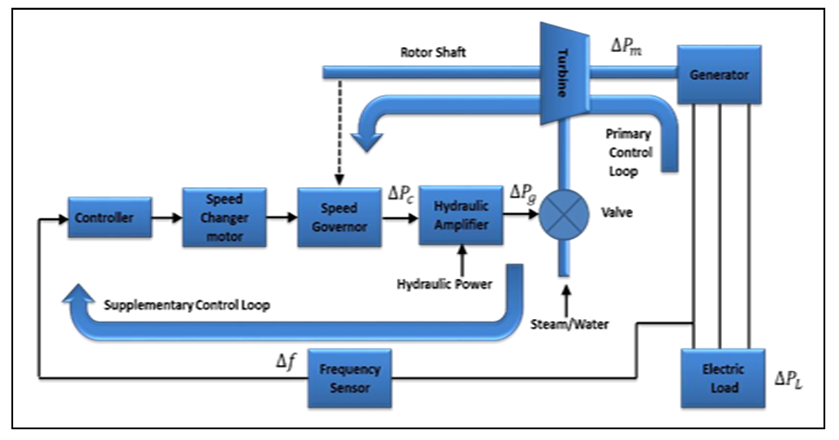Figure 1. Block diagram of the control loops of a synchronous generator [38]

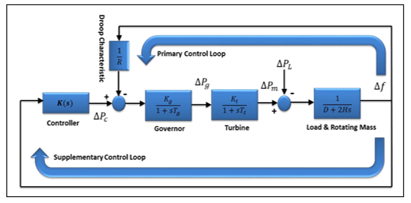Figure 2. Contol model of an AGC system with primary and secondary loops [38]

Having a realistic model considering physical constraints can significantly increase the accuracy of simulations. Therefore, physical constraints such as governor dead band, generation rate limit, and time delays are developed and added to the used AGC model.

In a multi-area power system in which different areas are connected through high-voltage transmission lines, a load change in one area will affect the frequency in all the other areas. Therefore, frequency deviations in an area may be the result of a power mismatch either in that area or the whole interconnection. Thus, in a multi-area power system, Area Control Error (ACE) is utilized in load frequency control (LFC) studies for achieving the power balance in interconnected control areas. ACE is a linear combination of frequency and net tie-lines power deviations, and maintaining it as close to zero as possible, can fulfill the objectives of AGC. Therefore, ACE can be a useful tool for AGC strategies. An ACE signal is computed according to each area’s frequency and tie-lines power flow deviations and is sent to the area’s controller to define the new set-point for each area [26]. Fig. 3 shows the AGC scheme in a multi-area.

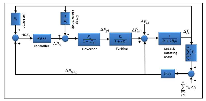Figure 3. AGC scheme in a multi-area power system [38]

2.2. AGC Nonlinearities and System Model

2.2.1. Dead-band of Speed Governor (GDB)

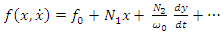
By allowing speed changes, the Speed Governor Dead Band prevents the governor control valves' position from shifting for a given position. The system response could be significantly impacted by the governor's dead band. The dead-band effect may be relevant because AGC research considers relatively tiny signals [27], [28].

Unintentional and intentional dead bands are the two main types of the dead band. Unavoidable and unadjustable mechanical effects of a turbine-governor system, such as stuck valves, sloppy gears, and hydraulic system nonlinearity, are referred to as the accidental dead band [29]. Modern governor designs use a dead band to reduce unnecessary controller activity and turbine mechanical wear for typical frequency changes in the power system. The turbine governor would not react to a system frequency excursion until the predetermined deliberate dead band was reached. Therefore, a greater frequency deviation results from the governor's Deadband. There are two ways to implement dead bands: step-function and no-step-function, respectively.

The first kind causes an abrupt change in mechanical set-point, which is undesirable since it causes excessive loads on mechanical components [30].

The GDB produces a continuous sinusoidal oscillation of a natural period of about T_S = 2s [31], [32]. The nonlinearity of the hysteresis is defined as,

(1)

there, x is taken as a sinusoidal oscillation with f₀ = 0.5 Hz and can be expressed as:

(2)

Since the dead-band nonlinearity tends to give continuous sinusoidal oscillation, such an assumption is quite realistic. Then, the F function can be evaluated as a Fourier series as follows:

(3)

Where and ……………. are the Fourier coefficients.

It is sufficient to think about the first three terms for an approximation (3). is equal to zero because the dead-band nonlinearity is symmetrical about the origin.

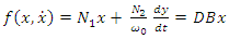(4)

where DB stands for the dead band. The parameters of the dead-band nonlinearity are established in this work using literature [33], [34], [35], [36]. The analysis's findings allow for the transfer function of the governor with dead-band nonlinearity to be stated in (5).

(5)

2.2.2. Generation Rate Constraints (GRC)

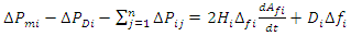
GRC limits the generating output change rate, which restricts AGC systems. Without this restriction, when AGC systems are vulnerable to significant transient disturbances, the controller may experience unnecessary wear and tear. The generation rate change is restricted as GRCs are implemented, which causes significant ACE variations. As a result, compared to situations when the generation rate is unrestricted, the length of power imports increases dramatically [29]. Therefore, it is important to understand and take into account the role that GRC plays in the AGC. The mathematical formulation of the GRC effect is as follows:

(6)

Where is the mechanical output of the turbine at a given time window

2.2.3. Transportation Time Delay (ΔT)

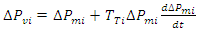
Delays in the mechanical system's response time and delays in the communication system both contribute to delays in the AGC systems. Transducer delays, the size of the discrete Fourier transformation window, processing times, multiplexing and transitions, the data size of the sensor output, and the type of communication channels being utilized are all contributors to time delays in AGC systems. These elements are described in depth [37], [38].

(7)

Where

(8)

Where

(9)

(10)

(11)

(12)

Where:

Table 2. Definition of parameters

2.3. Effect of Nonlinearities on AGC Operation

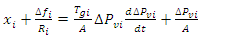
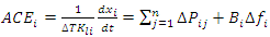
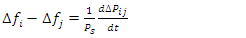
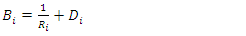
To sustain intended power exchanges across tie lines in an interconnected system with two or more control areas, each area's generation must also be managed in addition to frequency (inter-area transmission lines). The term "load-frequency control" refers to the regulation of both frequency and generation. A single-generation unit only has secondary control over a certain area, while each generation unit has primary control over a different one [39]. Load-frequency control is made possible by fusing distributed primary control with centralized secondary control. AGC is occasionally referred to as automated load-frequency control (vs. manual), or even the full frequency control system [40]. AGC is a crucial component of a power plant's "central nervous system."The energy management system (EMS) grid is conceivably the only automatic closed loop connecting the control area's IT and power systems [41].

Over-frequency and under-frequency protection relays activate tripping logic specified by a protection plan that differs from operator to operator when the system frequency exceeds a predetermined threshold and deviates from the nominal frequency (50 Hz for Zambia, as the majority of the rest of Southern Africa). Assuming a nominal frequency of 50 Hz, over-frequency relays begin tripping hydropower and thermal plants when the frequency rise exceeds 2.0% at all times (49 Hz to 51 Hz) for islanded networks, 5.0% at all times (47.5 Hz to 52.5 Hz) [42]. However, these relays are typically configured to tolerate deviations brought on by post-fault transients for brief periods. The only issue in our analysis is under-frequency load shedding (UFLS), which is carried out by under-frequency relays and causes a demonstrable loss in direct revenue. We use Mullen's UFLS scheme [41] for this study.

The basic idea behind the plan is to shed this much load when the system frequency decreases by more than 0.35 Hz below the nominal frequency:

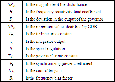
Where is the change in the generator's mechanical power, is the change in the generator's electrical power, and R is the characteristic. To cause the power supplier to lose money, an attacker can try to introduce fake data into the autonomous generation controller in the hopes of causing load shedding. Our goal is to characterize and quantify these risks.

For this work, we used the two-area AGC system model and associated simulation parameters [43]. The automatic generation controller is an integral controller of gain AGC design is an established discipline with designs dating back to the 1950s; a simple integral controller seems to be a logical starting point. The UFLS relay in each area decides on the necessity to shed load, and the amount of load to shed if necessary, using Mullen’s algorithm [43]. Once the system frequency has stabilized for at least 30 s, the UFLS relays reconnect the shed loads in the reverse order they were shed.

In this sample configuration, the maximum sheddable loads are capped at 4 p.u. and 1 p.u. for areas 1 and 2 respectively. “p.u.” stands for “per unit” and is simply the ratio of an absolute value in some unit to a base/reference value in the same unit. The base load for both areas is taken to be 1000 MW.

3. Methodology

3.1. Long Short-Term Memory (LSTM) Model

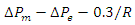
The fundamental concept behind the implementation of machine learning techniques in attack detection is that normal data and modified data tend to have a certain distinction in the projected space. This data together with the historical data can be used to develop the learning model to detect the anomaly. But the challenge remains due to the vast volume and the larger dimension of data to be trained. As the power grid is growing and the dimension of measurement variables has increased tremendously, the selection of the data learning techniques is largely dependent on the computational complexity, convergence rate, training loss, and training duration. LSTM is a unique technique to facilitate the data learning process. A multilayered LSTM framework as shown in the figure can capture the uncertainty of the modern grid and can successfully detect the presence of cyber anomalies [44].

Different length input data sequences can be handled by LSTM networks. Sequences are padded, truncated, or divided before being sent over the network to ensure that each sequence in each mini-batch has the required length (cells) [44–45]. A simple LSTM network for regression is depicted in figure 4 below. An input sequence layer and an LSTM layer make up the LSTM network's core. Time series data are fed into the network via the input layer, and afterward, long-term relationships between the input time steps of the sequence data are found by the LSTM layers [44], [45].

Figure 4. The LSTM network for regression

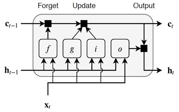
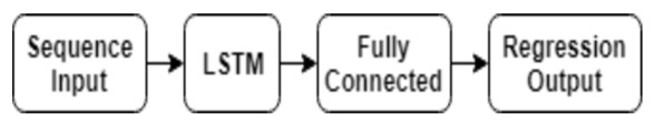
At every time step, the input measurements vector is passed through the LSTM block. There are three inputs to the LSTM cell: previous timestep (t-1) hidden state value, previous timestep (t-1) cell state value and current timestep (t) input value. The learnable weights of an LSTM layer are the input weight W, the recurrent weight R, and the bias b, see figure 5. The matrices are concatenated as follows [45]:

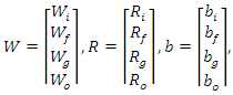
Figure 5. Flow diagram of the LSTM block at time step t

There are four dense layers: Input gate , Forget gate , Cell candidate and Output gate . The model uses a multi-class classifier model with four output labels. The output state of the LSTM block at every time step is used as input to the model for the next time cycle. The block applies a cell policy to limit the number of time steps and data points. The cell consists of an input gate, forget gate, and a control gate. The input gate is responsible to decide which values to be updated. The forget gate decides the number of data points to be used in the calculation and the control gate outputs the control variable using the output function. The cell state at time step is given by element-wise multiplication as [44],

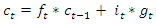(13)

(14)

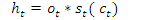
Where, is the state activation vector which is a function of cell state time. Every four dense layers are expressed as the function of t as,

The gate activation vector can be expressed using the sigmoid function as 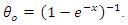The measurement matrices and the adjustable weight matrix are trained with the LSTM model for attack surface detection. The training of data is based on different input parameters: input layers, hidden layers, hidden units, dropout, sequence length, batch size, learning rate, optimizer, FC layers, and output layers. We can stack each LSTM layer on top of the other so that the output of the first LSTM layer is the input to the second LSTM layer. The hidden layer defines the number of LSTM layers stacked on top of each other. The dropout parameter controls the data fitting sequence. Sequence length defines the number of samples that follows the current in the sequence [44].

The prediction from the classifier model is studied for four possible outcomes of output labels.

i) True Positive (TP): positive prediction with positive ground truth,

ii) True Negative (TN): negative prediction with negative ground truth,

iii) False Positive (FP): positive prediction with negative ground truth,

iv) False Negative (FN): negative prediction with positive ground truth

The outcomes of the classification model are observed using four key metrics.

i) Accuracy metrics: These represent the correctness of the positive and negative classification.

ii) Precision metrics: These represent the correctness of the positive classification.

iii) Recall metrics: These indicate the ability to predict positive cases.

iv) F1 score: This metric correlates between precision and recall.

3.2. Attack Detection and Mitigation

For challenges involving classification and regression, LSTM structures can be used. The type of output— continuous (prediction) or discrete—is determined by the last layer activation function (classification). Attack detection is carried out by using the softmax function in the output layer to provide discrete outputs (labels) [46]. First, we train the LSTM_detection model, a multi-class classifier model with four output labels (normal state (NS), and to identify the attacks. The predictions of a classification model are evaluated for each of the four possible outputs, by considering an output l as positive and all other outputs as negative [47]:

i) True Positive (TP): positive prediction with positive ground truth,

ii) True Negative (TN): negative prediction with negative ground truth,

iii) False Positive (FP): positive prediction with negative ground truth, and

iv) False Negative (FN): negative prediction with positive ground truth. Accordingly, the following four statistical metrics are used:

(15)

(16)

(17)

(18)

where accuracy serves as a general metric of model success by estimating the chance of accurate classifications (both positive and negative); Recall estimates the likelihood that all positive labels will be correctly classified, and it serves as a gauge of the capacity to forecast positive cases. The precision and recall are balanced out by the score. The accuracy metric assesses the likelihood of correctly classifying positive cases and serves as a gauge of confidence in the anticipated positive cases [47].

Second, we develop the LSTM_mitigation regression model to reduce the impact of attacks that are detected. To forecast the proper signal values based on the other uncompromised signal data, we build and train a model for each of the system signals. When the system is in operation, only attacks that have been detected by the LSTM_detection model will cause the appropriate mitigation model to be triggered. Since LSTM_mitigation is a regression model that forecasts the attack measurement's continuous value to lessen the impact of the attack, its LSTM_mitigation is assessed using the attack mitigation plots and the root mean square error (RMSE) metric [47].

The control center processes frequency deviation and tie-line power readings from the N-Area AGC to compute the AGC signals that are delivered back to the areas. Fig. 6 shows the proposed detection and mitigation framework. The deviation frequency measurements [∆f₁, · · ·,∆f_N] from the N areas and the M tie-line measurements [P_tie1, · · ·, P_tieM] are included in the input features vector. Second, the LSTM_detection model receives these input properties to detect any attacks. If an attack event is discovered, the attacked measurement is located, and the associated LSTMitigation model is applied to lessen the impact of the attack on the attacked measurement. As a result, we will have (N + M + 1) models for a control center that monitors N locations with M tie-line power interconnections: a single LSTM detection model, (N + M) LSTM_mitigation models (one for each measurement). Based on the trusted and corrected signals, the control center calculates and sends back the new operation (OP) to each area [47].

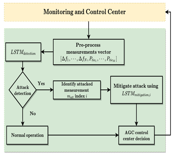Figure 6. Attacks detection and mitigation flowchart [47]

4. Results and Discussions

4.1. LSTM Models Training

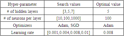
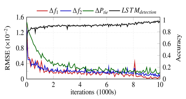
The two LSTM models are created and trained based on the formulation in Sections 3.1 and 3.2, and the datasets from [47]. To train and test the LSTM models, 2400 cases of attack scenarios (ramp, pulse) and normal operations are created and used as input data. Each case is composed of 1000 time steps vectors of the ∆f₁, ∆f₂, and ∆P_tie signals. Out of these 2400 cases, 70% were used for training and validation, and 30% were used for testing. The two models had one input layer, five hidden LSTM layers, and one output layer.

During training, the model performance is optimized by finding the optimal hyper-parameters. Hyperparameters include the number of hidden layers, the number of neurons per layer, and the learning rate. In this paper, we used the grid search technique [48] to tune the hyperparameters and to systematically search for the optimal number of hidden layers and nodes per layer. The optimal parameters are five hidden layers with 100 neurons per layer, the Adam optimizer [49] with a learning rate of 0.008. The grid search parameters and selected values are outlined in Table 3. The training of the models required 10,000 iterations for both the detection and mitigation models. Fig. 8 depicts the training progress for four models: one LSTM_detection model and three LSTM_mitigation models, one for each signal. The improvement for the detection model is measured by the increase in model accuracy performance on the testing data, while the improvement of the mitigation models is depicted by the decrease in root-mean-square error (RMSE) value for the testing data.

Table 3. Grid search parameters for tuning hyperparameters

Figure 7. RMSE of the 3 LSTMmitigation and accuracy of the LSTMdetection

Figure 8. Performance of the LSTMdetection model

4.2. LSTM Models Evaluation

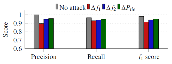
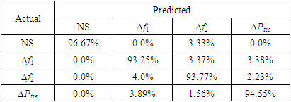
Table 4 shows the confusionmatrix for the LSTM_detection model. The confusion matrix is an important tool to measure the effectiveness of classification models, whether binary or multi-class models. The confusion matrix combines the actual outputs (ground truth), represented in the matrix rows, and the model predictions, represented in the matrix columns. For the LSTM_detection model, there are four output possibilities: No attack (NS), attack on ∆f₁, attack on ∆f₂, or attack on ∆P_tie. The diagonal elements correspond to the correct predictions, while the off-diagonal are incorrect predictions. For example, the model correctly detected and classified 93.25% of attacks on ∆f₁, and the remaining 6.75% were flagged as attacks but incorrectly classified. However, the model did not miss any attack case (i.e., flag an attack as NS), which is of greater importance to the system operator from a security perspective. The incorrect classifications are of small percentages compared to the correct classifications for all signals. In addition, Fig. 8 reveals the precision, recall, and f₁ score statistical metrics for each location output. The high scores in all three metrics (all above 90%) indicate that the LSTM_detection is a strong and balanced classifier.

Table 4. Confusion matrix for the LSTMdetection model

The evaluation of the LSTM_mitigation performance is achieved by analyzing the mitigated signals in comparison with the original signal as well as the attacked signal. Fig. 9 depicts a test case with an attack on ∆f₁. The graph shows how closely the LSTM prediction follows the actual signal, in contrast with the attacked signals as perceived by the system operator. Similarly, Fig. 10 and Fig. 11 depict a similar analysis of the ∆f₂ and ∆P_tie signals, respectively. Therefore, these signals obtained from the LSTM model can be used in case an attack is detected. The RMSE comparison between the magnitudes of attacked signals and the mitigated signals for all testing data is depicted in Fig. 12. As shown in the figure, the LSTM_mitigation model has significantly reduced the error in measurements.

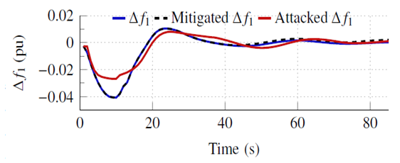Figure 9. Attack mitigation on ∆f1

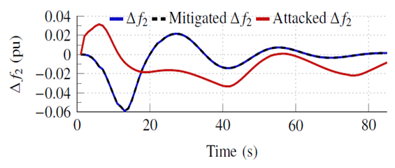Figure 10. Attack mitigation on ∆f2

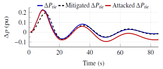Figure 11. Attack mitigation on ∆Ptie

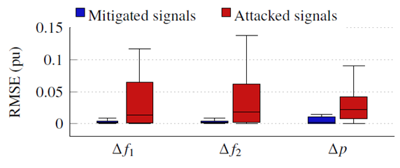Figure 12. RMSE of mitigated and attacked signals

5. Conclusions and Future Work

In large power networks with multiple areas sharing power, automatic generation control is a crucial controller. Cyber-physical attacks on AGC pose serious risks to the integrity of the entire power system since they give the attacker the ability to attack frequency and tie-line power signals in the communication system, leading to unneeded load shedding, power outages, and/or blackouts through the AGC. We model AGC nonlinearities and examine the potential vulnerabilities that could arise from neglecting them, in contrast to earlier efforts on AGC cyber-physical security. First, we demonstrated that if the nonlinearities are taken into account, the AGC's behavior and, subsequently, the control decision, differ. We showed that the linear AGC models that disregard nonlinearities do not provide appropriate defense against cyber-physical attacks that operate in the nonlinear region of the system. Second, we suggested and put into practice a two-stage strategy based on LSTM to identify and reduce the compromised signals to handle these threats. Its better performance in attack detection with good statistical metrics is confirmed by the examination of the detection model. The mitigation model can also improve the system's behavior and dramatically lower the RMSE of the attacked signals.

Future work includes expanding the risk analysis framework to include different types of coordinated attacks and comparing the impact expressed in different power system metrics. The mitigation techniques are based on Markov Decision Process (MDP) and Moving Target Defence (MTD). Finally, the attack resilient control framework should be enhanced to differentiate abnormal measurements due to cyber attacks from legitimate aberrations due to power system contingencies.

Future works include the intruders' decision to attack the AGC which is modeled over time using a Markov Decision Process (MDP). The research examines two tiers of the intruder's knowledge of potential power system situations. Taking into account the general scenario, where the intruder has less knowledge and uses a Markov Chain to describe the evolution of the system states, as well as the special case when the intruder can anticipate the future states for a brief time. In these two circumstances, the intruder's action process is defined as a finite-horizon MDP and an infinite-horizon MDP, respectively.

A mapping between power system states to the intruder's ideal actions (such as which buses to intrude on and what errors to inject) is the answer to the MDP. Based on the discovered attack strategy, the operator can additionally resolve the MPD and calculate the attack likelihood. When this happens, the operator can examine the susceptibility of specific parts and the effects of other variables (such as detection likelihood and system transition probabilities) on system vulnerability.