Kamal Gautam 1, Amarjit Singh 2
1Director of Engineering, rPlus Energies, Salt Lake City, UT, USA
2Honorary Faculty, Indian Institute of Technology, Guwahati, India; Professor, University of Hawaii at Manoa, Honolulu, Hawaii, USA
Correspondence to: Amarjit Singh , Honorary Faculty, Indian Institute of Technology, Guwahati, India; Professor, University of Hawaii at Manoa, Honolulu, Hawaii, USA.
| Email: |  |
Copyright © 2022 The Author(s). Published by Scientific & Academic Publishing.
This work is licensed under the Creative Commons Attribution International License (CC BY).
http://creativecommons.org/licenses/by/4.0/

Abstract
This paper aims to discover optimum economic conditions of purchasing a new personal automobile. The most important question answered is what percentage of the car’s purchase price should be paid as downpayment to minimize lifecycle costs for the economic benefit of the auto’ buyer and under what conditions. The life cycle cash flow of expenses and revenues was modeled using Excel to incorporate cradle to grave expenses and revenues that create a difference in comparing ownership costs. For this study, a 5-year period was considered as the ownership lifecycle, and three purchase options were analyzed to investigate the most economically attractive downpayment size. Various parameters such as mortgage rate, CD interest rate, and cost escalation rates were considered for forecasting future cash flows. The actual dollars were discounted based on the inflation rate to convert into real dollars at time zero, and subsequently projected to obtain the equal uniform net final monthly expense (EUNFME) -- the prime indicator of economic attractiveness. The analysis indicated that the lowest possible downpayment appeared to be the economically most attractive investment strategy for any option. A detailed analysis methodology is developed and presented.
Keywords:
Down payment, Mortgage rates, Inflation, Equal uniform net final monthly expense
Cite this paper: Kamal Gautam , Amarjit Singh , A Life-Cycle Cost Analysis for Automobile Purchase, International Journal of Inspiration & Resilience Economy, Vol. 6 No. 1, 2022, pp. 10-26. doi: 10.5923/j.ijire.20220601.02.
1. Introduction
Purchasing a personal automobile is a common decision process that most individuals encounter several times in their lifetime. The purchase of a vehicle is a significant economic event for the average wage earner, the economic decision for which must be made soundly. In addition, the automobile industry is extremely large in the United States, selling 17.5 million vehicles in 2016 (“The Number of Cars,” 2022); China produced more than 20 million vehicles in 2020 (“Production of Cars,” 2022); the auto industry in USA attained a total sales volume of $699 billion in 2005 (U.S. Dept. of Commerce, 2006), which became $81 billion during the Covid period in 2021 (“Car and Automobile,” 2021). It is the second largest household expense in the US after home mortgage (US Department of Labor 2006a), thereby indicating that the nation’s economy can be sensitive to sound and unsound decisions made by automobile purchasers en masse, making the economic analysis of car purchase and the considerations surrounding it a worthy topic of study. Indeed, car sales, in conjunction with home sales, are early indicators of the economy’s performance. Oftentimes, paying the maximum amount of downpayment on a car purchase is perceived to be an economically meaningful approach for the buyer. Still, spot surveys conducted by the authors revealed that buyers do not undertake a detailed economic life-cycle cost analysis to support their decision. This paper attempts to assess if paying the maximum amount of downpayment is attractive from a life cycle cost analysis point of view, and determine the optimum approach to investing in an automobile. The analysis seeks to inform potential buyers of the economic perspective of their decision.The life cycle cost analysis is an investment evaluation considering all cradle to grave expenses. All costs associated with and starting from concept (selection) and then spanning purchasing, operating, maintaining, and final disposal (resale) of the automobile make for its life cycle costs. All significant costs are considered in this paper to perform a reliable life cycle cost analysis that can be applied towards making practical economic decisions within the financing system in place in the United States. The calculations undertaken are based on calculated, recommended, and fixed data to achieve the paper’s objectives. However, the calculator prepared to undertake the analysis can easily accept user-fed, specific values in its input sheet.From an economic perspective, one of the most important factors is the time value of money, i.e., inflation. This factor is seldom considered in consumer decisions but can have a significant effect when the purchases become large, such as for an automobile or house. Thus, the impact of inflation is a cornerstone in this study. One of the major assumptions is that if the consumer were not to purchase an automobile, the consumer could spend that money on other consumer products – such as food and eating at restaurants, travel, leisure, etc. The consumer price index thus emerges as the index to use in determining the time value of money.Finally, this paper seeks to inform the millions of prospective automobile buyers of their economic interests while purchasing a personal automobile.
2. Objectives
The intent of this article is to establish a methodology to guide automobile buyers to arrive at the most economically attractive decision. Consequently, the prime objective of this paper is to investigate the most attractive downpayment size for auto purchase from the life-cycle cost point of view for a five-year ownership period1. Thus, the paper analyzes the combinations of mortgage and CD interest rates2 to find the most attractive downpayment. Hence, this article will ascertain whether the automobile mortgage rates influence the optimum decision in conjunction with a downpayment, coupled with considering the time value of money (inflation).
3. Literature Review
Normally, there are four basic methods of acquiring an automobile: some buyers borrow partially, some pay upfront fully, some borrow fully, and others lease the automobile. Traditionally, the American public prefers to own a new car in contrast to a used car, and Burgress (1999) reported that two-thirds of all new automobiles on the road are purchased while one-third are leased. However, Fan and Burton (2005) observed that published research on why auto buyers chose one method against another is rare. Since prices of new autos are rising faster than income, the length of loans has increased from two-three years to five-six years (Reed 2007; Solheim 2007). The issue of the economics of car purchase is not new. However, a continuing interest prevails on this topic due to many new car buyers in the market and their impact on the nation’s economy. According to a survey by Edmunds.com, the average down payment for a car in the United States is $2,400; the average amount financed is $24,864; and the average monthly payment is $479 (Solheim 2007). J. D. Power & Associates (Fortson 2007) found that the average rate funded by credit unions was 5.7%, while banks’ and automakers’ in-house financing loans averaged 6.8% and 5.3%, respectively, for a typical five-to-six-year loan term. These are raw statistics, which vary from year-to-year, and which tell us the situation on the ground, but little about what really helps the auto-buyer, the consumer, or how the consumers’ interests can be increased.Although leasing represents only one third of car ownership, recent years have witnessed an advance on economic research into leasing (Trocchi and Beatty 2003; Mannering et al. 2002; Miller 1995; Fan and Burton 2005; Patrick 1984). The belief that leasing comes free of ownership hassles is appealing to consumers. However, suppose good information was to be available on the real costs of ownership. In that case, consumers may realize that ownership has the opportunity to be cost-effective and more economic, accompanied with limited hassles till such time as the car is in reasonably worthy condition. This begs the questions of the life cycle costs for automobile purchase. It would be interesting to learn of consumer options concerning financing and down payment considering the time value of money. Essentially, one must ask the question: what amount of downpayment benefits the consumer most? What exactly are the real dollar expenses faced by the general auto’ buyer, even though any consumer can answer the question of what the major cost items are? The fact is that while auto’ salesmen, auto’ groups, and the auto’ industry talk a lot about selling more cars and what the latest gadgets are, they do not inform the consumer in detail of what buying strategy is most in the consumer’s economic interests. Thus, it is important to determine what actions really are in the consumer’s interest. This paper seeks to address that economic strategy via a few important variables that are downpayment, mortgage rates, CD rates, and inflation rate.
4. Methodology
The analysis involved in this paper is a six-step process of engineering economic analysis. It applies escalation rates to current prices, obtaining future expenses over the ownership period. Then, it deflates those future values to present value, thereby incorporating the effect of inflation. Once real dollars are thus obtained, the values are distributed over the ownership period to get the real monthly expenses. The steps are independent of the year of analysis. They are methodically explained below.Step 1: Establish the life-cycle cash flow. i. Determine ownership period, and the amount of loan to be borrowed. ii. Identify all expenses paid at the time of purchase, i.e., time zero. Normally, these expenses are down payment, registration, insurance, and other minor expenses that are due on the first day of ownership. iii. Identify all future ownership and driving-related recurring expenses until the ownership is terminated and automobile is disposed. All these expenses are identified and established based on the market rate at the time of auto’ purchase at time zero. These expenses are monthly mortgage, fuel costs, repair & maintenance (R&M) costs, insurance premium. Step 2: Establish interest, inflation (discount), price escalation, and depreciation rates. i. Establish Monthly mortgage rate (m%): This is done by surveying various banks, credit unions, mortgage lending companies, auto’ retailers, and automakers’ in-house financing institutions. ii. Establish Certificate of Deposit (CD) rate (k%): This is also accomplished by surveying various banking institutions. This rate will be used as a minimum attractive rate of return in the economic analysis. iii. Establish annual inflation rate (f%): The annual inflation rate is normally derived from the historical consumer price index (CPI). For this analysis, and as an example, historic data for consumer price index (CPI) for the period 1971 to 2006, viewed for urban consumers of the United States, was utilized (U.S. Department of Labor 2007b). Lognormal regression analysis was applied to this data for forecasting inflation rates and analyzed to forecast future price indices after deriving the regression equation using EXCEL3. Inflation rates are used for discounting future values into present worth real dollars. iv. Annual price escalation rates (e%): To generate the actual value of recurring expenses, reliable forecasting of future cash flows is necessary. For this purpose, historical data of all expense items have to be researched. For example, to forecast the future price of gasoline, it is necessary to gather historical price data of gasoline. Then, the historical data is regressed to establish the regression equation and thus derive future possible price escalations and prices. This process is repeated for all recurring expense items, as far as possible. v. Establish depreciation rate of the automobile (r%) to determine the asset’s salvage value. This was done in this paper by studying the estimated depreciation rates of various automobiles at Edmunds.com and by taking counsel from Caterpillar’s Performance Handbook (2004) for vehicle maintenance which provides information on the amount of money spent per year on maintenance as a percentage of the vehicle’s cost.Step 3: Calculate cash flows:i. Monthly mortgage (M) is calculated using the traditional engineering economy formula, M = P (A/P, m%, n), where M is in actual dollars, P = Amount of loan borrowed at the time of auto purchase, m = Mortgage interest rate, and n = number of interest periods. ii. Determine actual dollar values (FVi) of discrete future expense and revenue items identified in step 1 (iii) based on the escalation rates established in step 2 (iv). This generates a stream of future cash flow throughout the ownership period. Actual dollars at the end of each discrete time are calculated for each expense by utilizing the traditional engineering economy equation, FVi = B (Fi/P, e%, ni), where FVi = actual dollar value at a specific future time, B = Base line (Current) value of individual expense item, and e = escalation rate of the expense item under question.iii. Determine the resale value in actual dollars of the automobile at the end of the ownership period by utilizing the depreciation rate established in step 2 (v). Though, there are various methods for calculating depreciation, salvage value was calculated by straight-line depreciation. For simplicity 35% total depreciation was assumed4, which amounts to -8.25% per year compounded yearly.iv. Determine associated ownership termination (disposal) costs. For the purpose of this analysis, disposal cost was taken only as the advertising cost for resale. Step 4: Transform all future cash flows (FVi) into present worth (PVi).Now, transform all future cash flow (FVi - actual dollar values) into present worth (PVi - real dollar value) at time zero, considering the time value of money. For this purpose, use the generic engineering economy relationship, PVi = FVi (Pi/Fi, f%, ni), where f = Inflation rate (discount rate). Then, all the discrete PVi are summed by the formulation 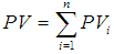 to determine the present worth of each expense item.Step 5: Determine EUME, EUMR and EUNFMEi. Once the PV is obtained in real dollars, the EUME (Equal Uniform Monthly Expense) is simply PV ÷ n. Stated in engineering economy terms, (EUME) is calculated for each expense item using the traditional engineering economy formula, EUME = PV (A/P, 0%, n), where A = equal uniform monthly expense amount, in real dollars, PV = present value in real dollars of each expense item calculated in step 4, and n = number of interest periods for the given expense item. Then sum PV of all expense items to find the total EUME. ii. Equal Uniform Monthly Return (EUMR) is calculated as follows:Subtract the resale advertisement cost (actual $) established in step 3 (iv) from the salvage value (actual $) determined in step 3 (iii) to find net future return in actual $. Convert the net future return (actual $) into present value (real $) by utilizing the generic engineering economic relationship PV = FV(P/F,f%,n). Further, subtract the downpayment amount from this present value, and then simply divide the resulting amount by number of months (n) to find EUMR. iii. The equal uniform net final monthly expense (EUNFME) is the difference between the EUME and EUMR. EUNFME measures “inflation-free” present value that incorporates all cradle to grave expense items for the entire ownership period distributed equally over each month. This is the decision-making parameter being sought. In this study, EUNFME is taken as the measure of investment attractiveness. The smaller the EUNFME, the better the investment deal. Step 6: Perform sensitivity analysisSensitivity analysis is performed against down payment, CD, and mortgage rates at varied intervals to understand their effect on EUNFME. These intervals are defined later in the body of the article and in Table 2.A flow-chart of the methodology is shown in Figure 1.
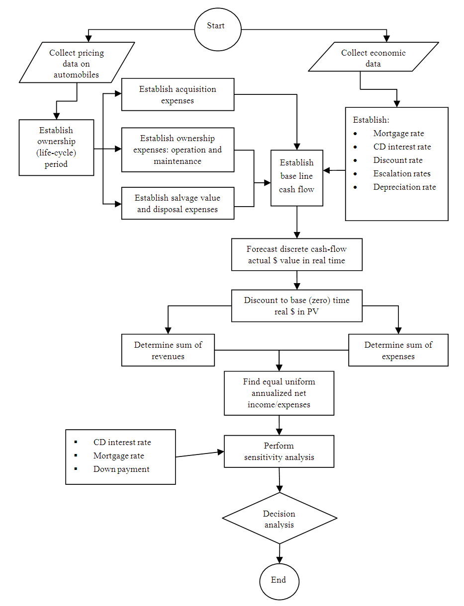 | Figure 1. Flow-Chart of the Methodology |
5. Essential Variables
The essential expense variables include the obvious and not-so-obvious items. The obvious items are mortgage, repair and maintenance (R&M), insurance, registration, and fuel. The not-so-obvious items, which are often ignored or overlooked by consumers, are the loss in interest of investments and expenses incurred at time zero and other periods. Another major item is the inflation rate, which markedly affects the present worth analysis and must always be included in realistic decisions. Finally, price escalation is another important variable item that determines the future cash flow. The expense variables, mentioned in detail in Table 1, Figure 5, and Figure 6, are listed below. 1. Monthly Mortgage2. Recurring Registration cost3. Recurring R &M cost4. Recurring Insurance cost5. Recurring Fuel cost6. Loss of Interest on Down payment7. Loss of Interest on Registration Costs8. Loss of Interest on R &M Costs9. Loss of Interest on Insurance Costs10. Loss of Interest on Fuel Costs11. Saved income tax on lost interest The essential processes during the time of selling (or trading-in) the vehicle include paying off the remaining loan (which is usually paid off in any case since the loan period coincides with the ownership period in our example), the resale value of the vehicle (the only revenue item in the entire stream of data analyzed), and disposal costs incurred. Balances are calculated at the end of the ownership period. The major items at the time of resale and used in Figure 6 are listed below:1. Salvage value2. Advertisement cost3. Principal amount to be paid back to bank4. Balance after selling
6. Scope and Assumptions
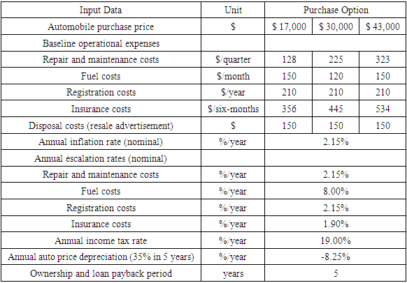
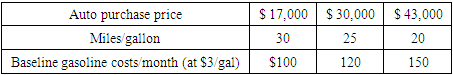
To evaluate various conditions, and investigate the most attractive downpayment, it was necessary to approach the analysis with some realistic assumptions of expenses. As a first step, three typical purchase prices are assumed -- $17,000, $30,000, and $43,0005 -- which reasonably cover the breadth of passenger cars in the USA. The ownership period is assumed to be five years, since that is the general mortgage period for auto’ financing, and also because many cars reach the end of their useful life in five years if driven excessively. Annual registration cost is considered equal for all car types6. However, the annual insurance premium is different based on the initial purchase price, the calculation of which is explained later in the price escalation section on auto’ insurance. Annual repair and maintenance costs are taken as 3% of the auto’ price7. The auto’ resale or disposal cost is taken as $150 at time zero as present value, representing the advertising cost in a local newspaper in a major city. In making a decision to achieve our objectives, several uncertainties are inherent such as the fluctuation of CD interest rates, inflation rate, fuel costs, and R&M costs. To consider practical approaches to car purchase and money investment, the CD interest rate was fixed as being the available rate for five years at the time of purchase. The auto price is depreciated by 35% in five years, distributed linearly, based on the Kelley Blue Book recommendation (Kelley, 2007). To complete the analysis, the set of input data relevant for three purchase options used in this paper are tabulated in Table 1. The variable input data range is summarized in Table 2. Table 1. Constant Input Data for Three Purchase Options (Present Value at Year Time Zero)
 |
| |
|
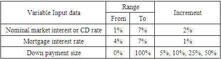
Table 2. Variable Input Data for All Purchase Options
 |
| |
|
Finally, the analysis is limited to purchasing a personal automobile by an individual, in contrast to a purchase by a company or corporation that may have tax write-offs. Moreover, simple mortgage considerations are as those prevalent in the USA. For simplicity and convenience, in the example and in the paper, the base present time for economic analysis is assumed to be December 31, 2007. Thus the 5-year ownership period would end on December 31, 2012. It is important to fix a start date in the analysis to apply escalation regression equations consistently.While reasonable values for expenses and escalation rates for all parameters were assumed in this study, the user can input his or her precise data in the Excel program prepared to arrive at the precise EUNFME, since there are variations in the values assumed from state to state, and city to city. It is not possible to capture all the data for all states and cities in a general formula. Correspondingly, particular calculations have to be calculated independently. Moreover, the scope of this study was limited to sensitivity analysis of down payment, mortgage rate and CD interest rates only. Variable parameters of life cycle costing such as inflation rate and escalation rate are evaluated based on a specific model dependent on logarithmic regression. However, other forecasting models can be used, as can those that adopt a portfolio approach to forecasting (refer Singh 2006) for a project cost forecasting model using the portfolio approach). The automobile depreciation rate was also assumed fixed8, when, in reality, all the thousands of models of cars available in the United States could have depreciation rates anywhere between 25% and 65% of the purchase price (Johnston 2006; Kelley 2007). Similarly, longer ownership periods may be cheaper because of smaller real dollar mortgage amounts if repair and maintenance do not leap higher. Still, this analysis was limited to a five-year ownership period with the belief that the five-year point is critical from many perspectives9 and provides realistic numbers for equipment management. However, alternate ownership periods can be programmed. For a much deeper understanding of EUNFME, sensitivity analysis of ALL the variables can be undertaken, but this is absolutely beyond the scope of this paper, perhaps impractical, and might instead complicate and confuse the buyer’s or consumer’s interests. Correspondingly, this paper is focused on providing the buyer with a realistic economic option and analysis for auto’ purchase.
7. Inflation / Deflation Rate
To make the economic analysis realistic, historical data of the Consumer Price Index (CPI) was obtained for the period 1971-2006, with the base year being 1982-1984 (US Department of Labor 2007b). 1971 was taken as the cut off CPI data point, when the US economy entered into the gold standard. The CPI indices for years 1971 and 2006 were 0.405 and 2.013 respectively. Considering annual compounding from 1971 to 2006, the annual average CPI inflation rate was found to be 4.69%. However, a lognormal regression generates the best-fit line to historical data with a correlation coefficient, r2 = 0.99, as shown in Figure 2. The regression equation is generally more representative of future trends than past year-over-year averages, mainly because the regression follows past trends. The user of the calculator developed in this study can enter his/her own preferred inflation rate. Thus, based on the regression forecast, the annual discount rate of 2.15% was used in the analysis as a measure of future inflation/deflation. 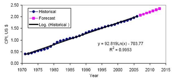 | Figure 2. Consumer Price Index (CPI) Regression and Forecast |
The regression for forecasting uses the time series data as explained above. However, the methodology developed is independent of the country or region or time period analyzed. This methodology can be applied to extend the time series data or use a different time series for a different country or region. The future applications will require new time series data for all parameters regressed, such as gasoline price and auto insurance premiums.
8. Price Escalation
The actual future prices of consumption items must be determined as accurately as possible to get a reliable idea of life cycle costs. The fact is that life cycle costs can never be 100% accurate if future costs are not known precisely, but it is never possible to predict future costs precisely. Thus, the best that can be done is to make progressions of past trends to arrive at future costs. Of course, there are different models – simple and complex -- for predicting future trends, but no one model can be used in all cases. In this study, the authors adopted the following methods for the items mentioned: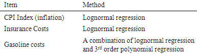 Repair and Maintenance escalation, as well as Registration costs, were taken equal to the inflation rate. For one, the registration expense is small indeed and can be assumed to climb at the inflation index to save effort in making needless calculations. The authors believe that R& M costs are closely tied to inflation since it is a direct function of the CPI and producer price index (PPI) (Singh and Gautam 2007).
9. Price Escalation: Auto Insurance Premium
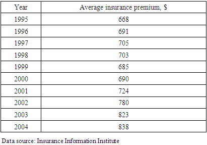
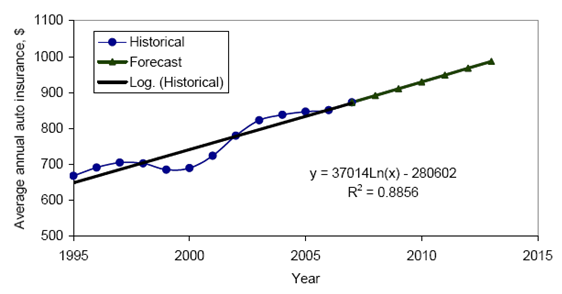
The insurance premium varies, depending upon the insurance company and the type of coverage subscribed by the auto owner in a particular locality. According to data published by The National Association of Insurance Commissioners, the average expenditure for auto insurance in the United States during the period of 1995 to 2006 was as shown in Table 3 (Insurance Information Institute 2006). A best-fit line was given by a lognormal regression (r2 = 0.8931) of the historical data, as shown in Figure 3. Table 3. Average Auto Insurance Premium in USA
 |
| |
|
 | Figure 3. Auto Insurance Premium Regression and Forecast |
Based on the forecast, the average annual insurance price escalation was calculated to be 2.09% during the five-year ownership period of 2007 - 2012. This escalation rate was applied to the current actual annual premium cost of $890 for 2007, and used to forecast future insurance expenses, as shown in Figure 3. To differentiate between the insurance premiums of the three different automobiles based on their original purchase prices options, the following procedure was adopted: The average annual insurance premium ($890) was directly applied to the purchase price option of $30,000. Then, 80% of the average premium was adopted for the lowest purchase price option ($17,000) whereas 120% of the average premium was adopted for the most expensive purchase option ($43,000). This is because more expensive cars generally have higher insurance premiums, though variations were found among different insurance companies. Nevertheless, fitting all insurance variations into a formula was discovered to be an impossible task. Thus, the baseline annual insurance premium assumed was $712, $890, and $1086 for the original purchase prices of 17,000, 30,000, and 43,000 respectively. It is an accepted practice to pay the insurance premium on a six-monthly basis, and therefore it was assumed as paid on a six-monthly basis in this life cycle cost analysis.
10. Price Escalation: Gasoline
It was assumed that the average miles driven per month are 1000. It was further assumed that fuel consumption for each type of automobile varies, which is quite obvious. The more expensive the car, the heavier its body and larger its engine size, resulting in higher gasoline consumption. Based on this assumption, fuel consumption rate is developed for this analysis as shown in Table 4. Table 4. Miles/Gallon for Each Type of Automobile (Assumed)
 |
| |
|
The historical data of Annual Average Gasoline Retails Sales Price (Energy Information Administration, 2007) was available from 1978-2006, which was used as a basis for forecasting. Considering annual compounding from 1978 to 2006, the annual average national price escalation of gasoline was seen to be 5.43% for the period of 1978 - 2006. A lognormal regression of the historical data yielded the following equation with a low correlation coefficient, r2 = 0.28: 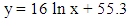 | (1) |
Where y is the gasoline price in cents/gal, and x is the serial number of years starting with 1 for 1978. But this correlation coefficient of 0.28 is extremely low and does not give credence to the significance of the regression. In addition, the log normal equation yields less than 1% average annual escalation on gasoline price, for the period 1978-2006, while the actual value was 5.43%. Therefore, the lognormal regression alone was not considered reliable for forecasting gasoline price. A third-degree polynomial regression provides the best-fit line to historical data with a correlation coefficient, r2 = 0.84, provided by the following equation:  | (2) |
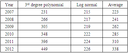
However, the third-degree polynomial yields a rapidly increasing price hike, and the authors considered such a forecast potentially misleading. The difficulty is that no other simple model can provide a reasonable answer, not to mention that gasoline prices are deeply linked to world politics, which is immensely uncertain. Therefore, for this paper, a judgmental approach was taken to forecast gasoline prices by taking the average of the lognormal and the third-degree polynomial equation, as shown in Figure 4. The calculation results are presented in Table 5. In this way, the final forecast generates an annual average price escalation of 8%. Considering the volatility of gas prices, an 8% annual price escalation rate was accepted for further use. However, it has to be noted that the accuracy of the gasoline price forecast is beyond the scope of this paper. Sensitivity analysis revealed that gas price escalation of 1% per year to 12% per year had no impact on the final recommendation regarding downpayment.Table 5. Forecast of Gasoline Price
 |
| |
|
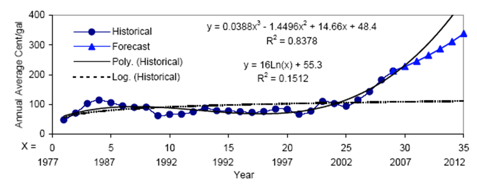 | Figure 4. Gasoline Retail Price Regression and Forecast |
11. Using the Calculator: The Excel Program
The cost analysis was programmed in Excel and automated for easy input and output review. The worksheet for data input and the resulting output was organized and set up as shown in Figure 5. This program utilized 13 Excel worksheets, and an outlook of the summary cost analysis sheet was organized as shown in Figure 6. 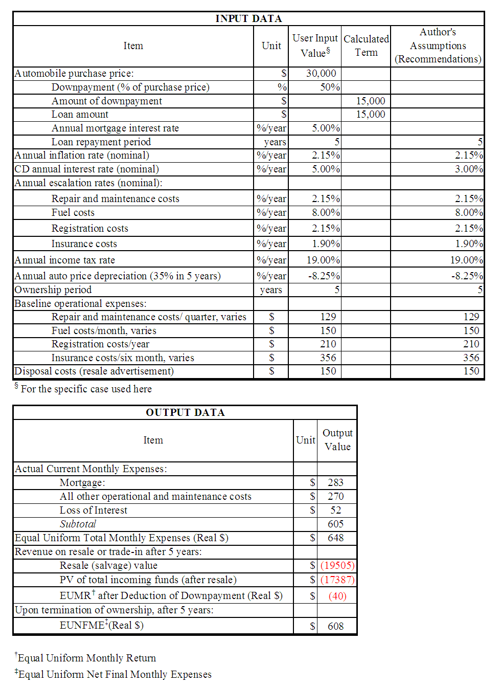 | Figure 5. Auto Purchase Excel Program Input Worksheet and Output Data |
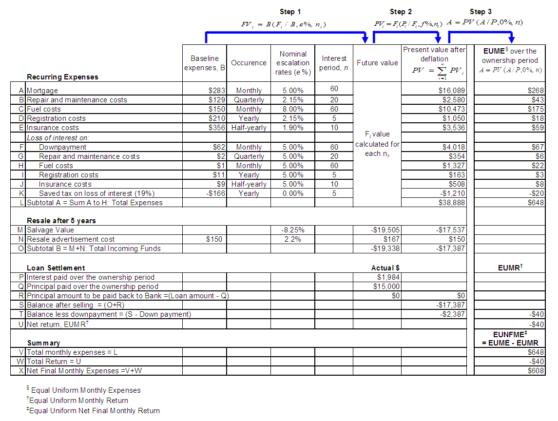 | Figure 6. Auto Purchase Cost Analysis Summary Sheet |
It is to be noted that the Excel calculator is very user-friendly. The user can enter any preferred value in the input menu and immediately find the resulting EUNFME in the output menu on the same worksheet. Thus, users can conduct their own sensitivity analysis and evaluate their own particular scenario in their part of the country. The data used (recommended) by the authors based on their study is provided in Figure 5 in the input menu. The specific input data adopted for this study is provided as shown in Tables 1, 2, and 4. To obtain graphs of effect of downpayment, mortgage rate, and CD rates, the downpayment was calculated for 5%, 10%, 25%, and 50% downpayment; CD rates were calculated for 1% to 7% at increments of 2%; the mortgage rate was calculated for 4% to 7% at intervals of 1% (See Table 2).
12. Results and Analysis
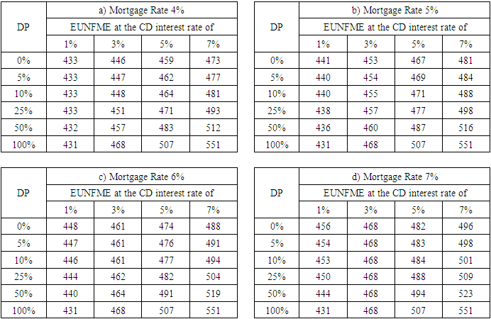
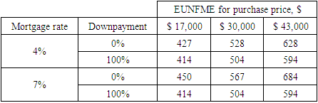
The output of the Excel program from sensitivity analysis of various conditions is summarized in Tables 6, 7 and 8, grouped by purchase price category. Utilizing the Excel output, various graphs were drawn for better visual observation and results, presented in Figures 7, 8 and 9, and discussed below. Moreover, for visualizing the actual transactions and their equivalent real $ values, representative cash-flow diagrams are drawn in Figures 10 to 12.Table 6. EUNFME for Purchase Price $ 17,000 for Various Mortgage Rates and CD Rates
 |
| |
|
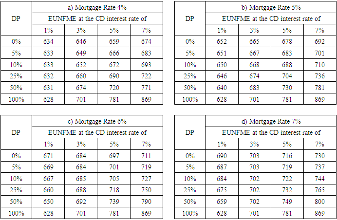
Table 7. EUNFME for Purchase Price $ 30,000 for Various Mortgage Rates and CD Rates
 |
| |
|
Table 8. EUNFME for Purchase Price $ 43,000 for Various Mortgage Rates and CD Rates
 |
| |
|
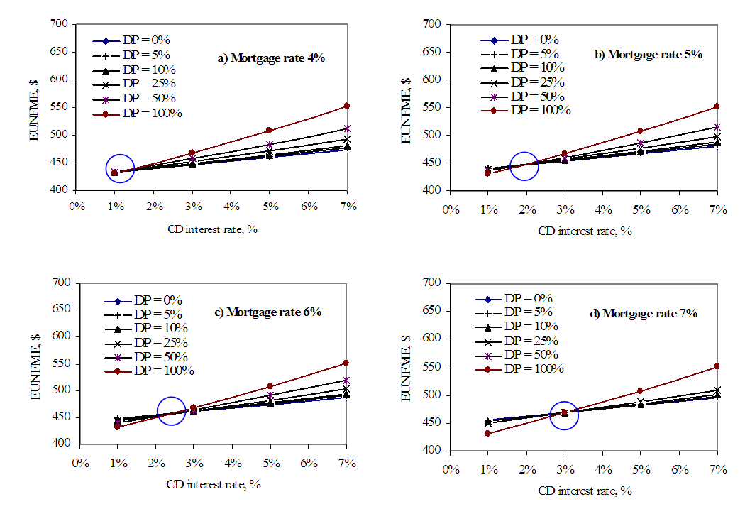 | Figure 7. EUNFME for Purchase Price of $17,000 |
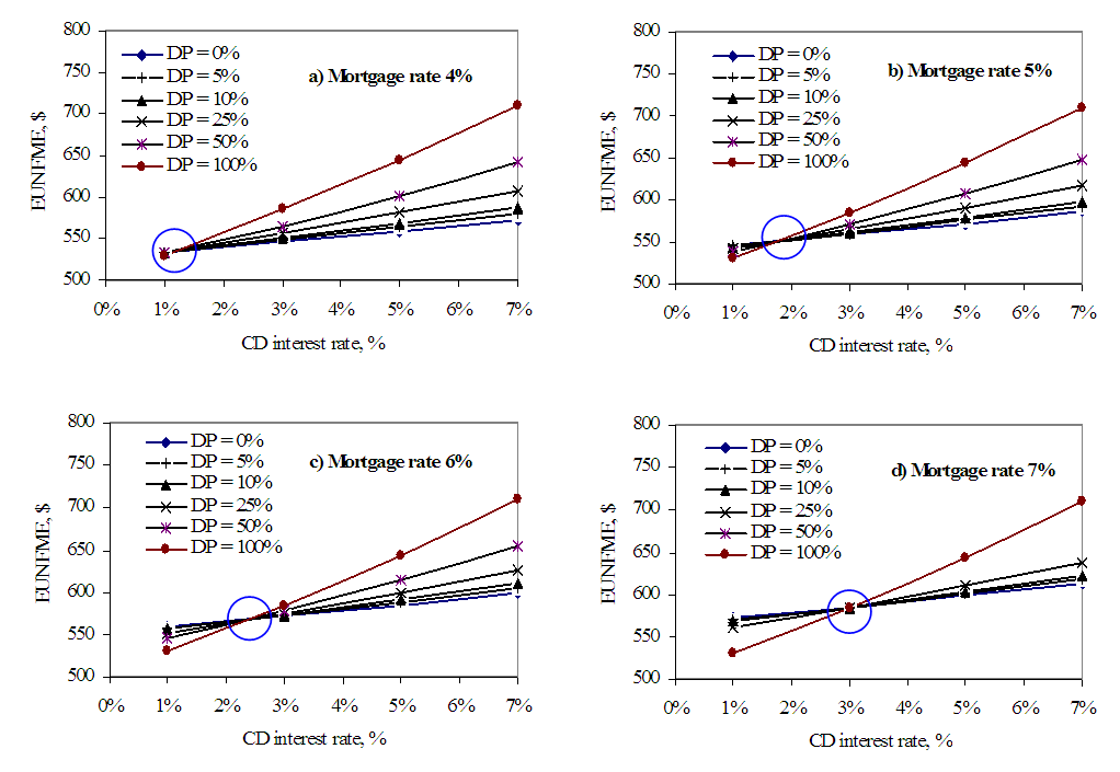 | Figure 8. EUNFME for Purchase Price of $30,000 |
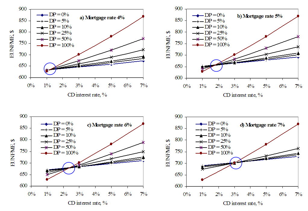 | Figure 9. EUNFME for Purchase Price of $43,000 |
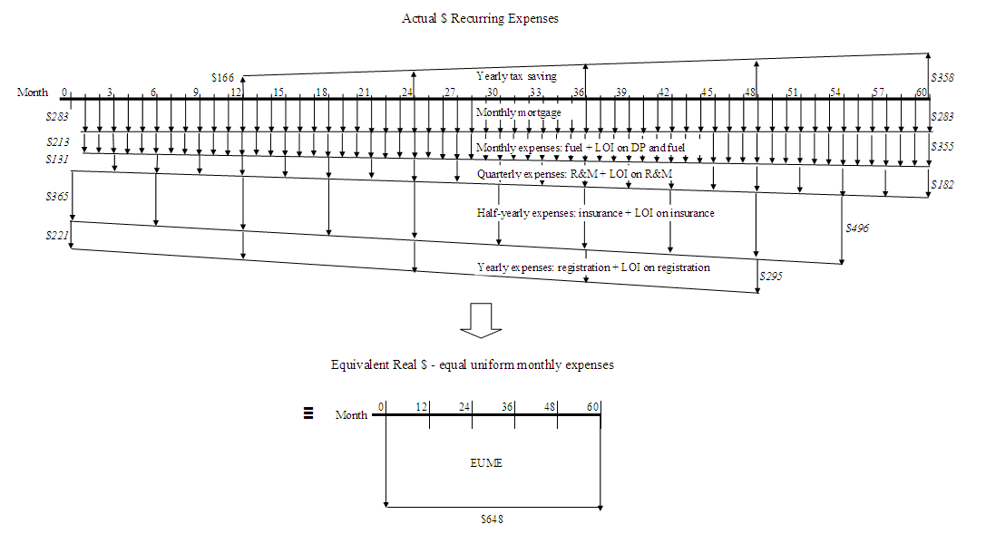 | Figure 10. Cash Flow of Recurring Expenses |
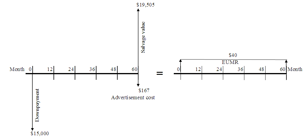 | Figure 11. Cash Flow Conciliation during Resale |
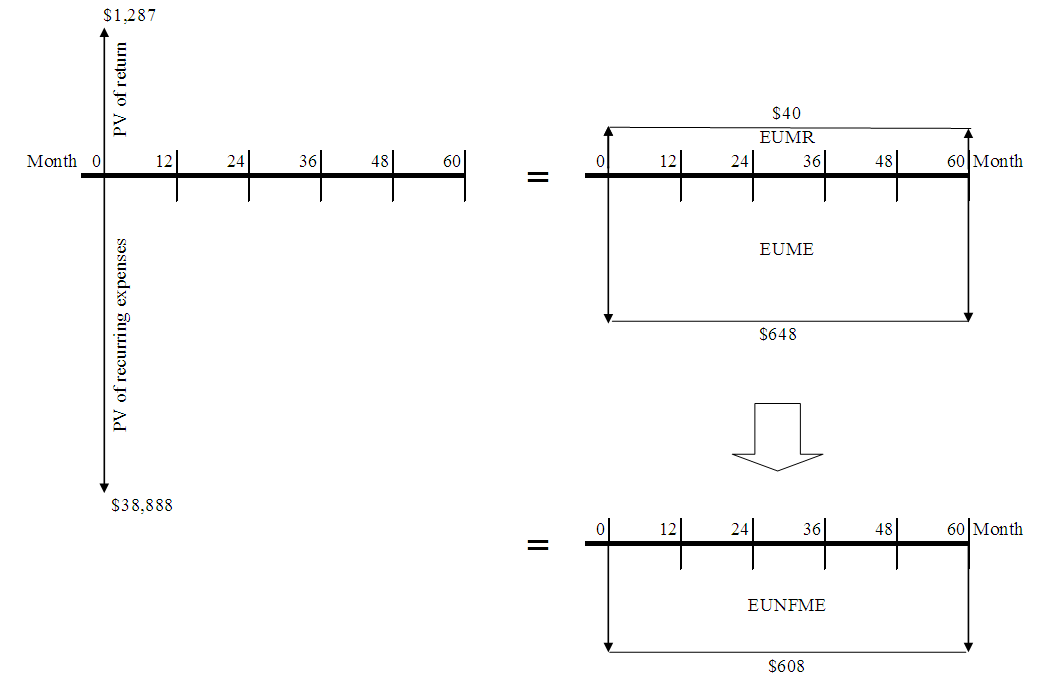 | Figure 12. Summary Cash Flow of all Expenses in Real $ - Equal Uniform Net Final Monthly Expenses |
13. Comparing Mortgage Rates
EUNFME increases as the mortgage rate increases. This sounds obvious, though reduced points with higher mortgage rates are often incorrectly assumed to minimize the impact on monthly mortgage expenses for home purchase (Singh and Gautam, 2007). From Figures 7, 8 and 9, it is consistently observed that the higher the mortgage rate for a selected CD interest rate and downpayment, the larger the EUNFME. The inflation effect is unable to reverse this trend.This trend is uniformly valid for all three purchase options, except for the special condition when the CD rate falls below 2%, 2.5% and 3% accompanied by 5%, 6% and 7% mortgage rates respectively. This brings us to analyzing the breakeven point where the EUNFME is the same at a particular CD and mortgage rates, irrespective of the downpayment (Figures 7 to 9). The breakeven point is marked by a circle in Figures 7 to 9. {Figures 7 to 9 should be read in conjunction with Tables 6 to 8}.
14. Breakeven EUNFME
The main factor in understanding the breakeven point is the particular effect on loss of interest on the lost opportunity of the auto’ buyer; coupled with the downpayment made at a finite mortgage rate, there is an effect on the EUNFME for a constant inflation rate. Very high CD rates will increase opportunity losses, but at low CD rates the effect can be less pronounced, such that paying a high downpayment starts to become increasingly attractive. The EUNFME decreases with lowered CD rate for all cases, but the slope of EUNFME v. CD rate increases with larger downpayment because of the particular influence of the magnitude of downpayment. At lower CD rates, the loss of interest of higher downpayment is higher. Still, the mortgage due to lower downpayment is even higher, thereby making the net monthly expense higher for low downpayment scenarios.At the breakeven point, it is apparent that making any downpayment is economically equivalent. Nevertheless, such a breakeven scenario is hard, perhaps impossible, to find in the real world. In addition, it has always been possible in the United States since WW II to find CD rates higher than the breakeven point rates, no matter what the prime lending rates. Normally, increases in mortgage rates are accompanied by increases in CD rates, and vice versa, from simple economic principles in the monetary system of economy management (Singh 1997).
15. Opportunity Loss: Comparing CD Interest Rates
EUNFME increases as the CD interest increases for a given mortgage rate and down payment. Thus, the actual loss of increased opportunity becomes more. When down payment is small, for example, 0% or 5%, the effect of CD interest on EUNFME is very negligible. But, as the downpayment increases, and as the buyer gives away more of his money at time zero, the opportunity loss through increased CD interest rates becomes more pronounced. Neglecting this opportunity loss during economic analysis is the biggest single flaw made by buyers and consumers and ill-informed auto’ salesmen and realtors (in the case of home purchase) not familiar with engineering economic analysis. However, buyers tend to overlook this item because it is a “hidden” cost item – not quite visible on the surface. It is seen that opportunity losses due to loss of interest amount to a considerable sum of money.
16. Comparing Down Payment Size
From Tables 6 to 8, EUNFME increases as the downpayment rate increases for any given mortgage rate and CD interest rates, for any purchase condition. This trend is associated with the opportunity loss mentioned in the previous sub-section. This trend is consistently apparent in Figures 7 to 9. From these tables and figures, it is observed that EUNFME has a linear relationship with downpayment for constant CD and mortgage interest rates. It follows that increased downpayment results in increased opportunity losses and is a major contributor to the reduction in net worth of the buyer.Interestingly, the maximum EUNFME for a given mortgage interest rate occurred when combined with the highest CD interest rate and the highest downpayment for all purchase conditions, as seen from Figures 7, 8, and 9. The lowest EUNFME occurred when the maximum downpayment was combined with the lowest CD rate, for all mortgage rates and purchase conditions. This means that varying the CD rates will have a profound impact on EUNFME. Thus, when the CD rate is the highest – such as 7% from our examples – the EUNFME is also the highest for any purchase price and any downpayment. In general, right of the breakeven point, EUNFME is highest when downpayment is 100%, and lowest when the downpayment is 0%. To the left of the breakeven point, however, this trend is reversed. The slope of the EUNFME v. downpayment profile becomes steeper as the mortgage rate is decreased for a constant CD interest rate. This means that the less the buyer borrows below the breakeven point, the better; conversely, the higher the buyer borrows above the breakeven point, the better.
17. Distribution of Recurring Expenses
It turns out that mortgage rate, downpayment, CD rate, and escalation and inflation rates are the primary factors affecting an appropriate automobile purchase decision. By rank order of contribution to expense, from the example provided in Figure 6, the order and weights of essential variables to the expenses (EUME) were:i. Mortgage rate, 40%ii. Fuel costs, 26%iii. Loss of interest, 16%iv. Insurance costs, 9%v. R&M costs, 6%vi. Registration costs, 3%Without considering the time value of money, i.e., by considering actual dollar instead of real dollars, the effect of fuel would be more pronounced; the same goes for mortgage. However, incorporating the time value of money yields a realistic picture of the effects of essential variables and lends reliability to the analysis.Without considering the loss of interest, the total expenses are less by 16%. A condition can arise with specific combinations of downpayment and mortgage rate where not considering this expense could falsely reveal that paying a mortgage is not attractive; for instance, Table 9 indicates that when loss of interest is not considered, the EUNFME for 100% downpayment is lesser than the EUNFME for 0% downpayment for all purchase price conditions.Table 9. EUNFME for Extreme Values of Downpayment when Loss of Interest is Ignored
 |
| |
|
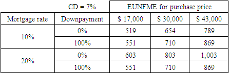
18. Sensitivity Analysis for Very High Mortgage Rates
What happens if mortgage rates were to increase enormously, such as up to 20%, a situation that occurred in the late 1970’s in the United States? Sensitivity analysis revealed that the effectiveness of downpayment again reversed itself. As Table 10 shows, paying 100% downpayment makes for a lower EUNFME than 0% downpayment for 7% CD rate. A CD rate of 7% was selected for this sensitivity because when prime lending rates are high, CD rates are also commensurately high.Table 10. EUNFME for High Mortgage Rates
 |
| |
|
Hence, it is interesting to observe that paying 100% downpayment is more advantageous at extremely low CD rates below the breakeven point or during very high mortgage rates that reach 20%.
19. Discussion
Given that this study determines that borrowing is more economic than paying 100% downpayment for realistic conditions when the economy is under control, who is it that isn’t happy with this finding? The lenders and bankers are happy because they get to lend more and make money. The consumer is happy because it is discovered that there is an economic advantage in borrowing, and the more the consumer borrows the better for him under the current inflation and lost opportunity conditions. The auto dealer is happy because now he can be assured that the buyer (consumer) will not wait until he accumulates savings towards a 100% downpayment, since the buyer can take out a loan by exercising leverage. The banks are also happy because the buyer leaves his equity in the bank rather than spending it on purchasing a car; alternately, the buyer can invest his liquidity in another investment of choice, thereby gaining the opportunity to multiply his assets. There does not seem to be a stakeholder that is not happy with the finding. Perhaps, the only counterargument is at a macro-economic level where it can be argued that the increased velocity of money might produce inflation, resulting in the consequent raising of borrowing rates.
20. Conclusions
From this analysis, it became clear that although paying the maximum downpayment might appear to be generally less burdensome to the lay consumer, it is not always the best investment decision from an economic perspective considering the time value of money and the combinations of CD and mortgage rates. The following conclusions can be drawn:1. Due to opportunity costs and inflation, the smallest possible downpayment was seen to be the most attractive investment decision for all practical considerations. 2. For each combination of mortgage and CD interest rate, there is a breakeven EUNFME that makes all downpayment options economically equivalent. However, this breakeven point occurs for extremely low CD rates that are not realistic. Hence, it is a good rule to adopt that the minimum downpayment should be made for all normal economic conditions.3. The analysis indicated that the investment decision is heavily dependent on the mortgage rate, opportunity loss of interest, and inflation rate, keeping in mind that the time-value of money is extremely important from the life cycle perspective. 4. The minimum downpayment is actually made possible considering the time value of money and opportunity loss of interest. When the opportunity loss of interest calculations are not considered, sensitivity analysis revealed that paying 100% downpayment was more attractive than taking a loan. However, such a calculation is a violation of the principles of life cycle cost analysis.5. Real dollar mortgage expenses were 40% of all expenses from the example provided. The opportunity loss of interest component is 16%, which is sizeable.6. For extremely high mortgage rates, 20% and higher, paying 100% downpayment was more attractive than taking a loan. Alternately, paying 100% downpayment was economically attractive for very low CD rates below the breakeven point.The study was conducted with certain assumptions, such as (i) 35% fixed depreciation, (ii) using logarithmic regression to forecast inflation and escalation rates, (ii) five-year ownership period, (iv) simple mortgage and certificate of deposit (CD) considerations prevalent in the United States, and (v) the vehicle would be purchased by an individual owner, in contrast to a corporation that may receive tax write-offs.Finally, the analysis methodology comprehensively considers all important meaningful parameters, representating the real economic results. This methodology is reliable since it considers the time value of money and lost opportunity costs. This research is important because the conclusions drawn here will help ordinary citizens to rationalize their investment decision whether to purchase or lease an automobile.
Notes
1. A five-year period is specifically chosen to match the normal loan period of a new vehicle. In addition, numerous vehicle owners trade-in their vehicle every five years, making it a sensible ownership period to evaluate. Moreover, many vehicles reach close to the end of their life in five years if driven extensively, making it even more reasonable to consider five years as an ownership period. Finally, the exact life of a vehicle is uncertain, thus compelling the researchers to use a reasonable life for this analysis.2. CD rates are used to calculate lost opportunity costs from loss of interest that the consumer might have otherwise gained if he were not to pay the downpayment or other expenses for the operation of the car.3. All regression analysis in this article was undertaken using the EXCEL program.4. Cars with excellent manufacturing quality and good consumer appeal tend to have a high resale value of around 65% of purchase price after five years, provided the cars are maintained properly and are in excellent condition at time of resale (Kelley, 2007). The authors have opted to follow the depreciation rate of such vehicles rather than considering variable depreciation rates, since the final decision should not be affected as a result.5. These three prices represent a small, economy car; a large Sedan; and a luxury SUV.6. Many states have equal registration costs for cars of all sizes.7. This is a reasonable R&M rate for passenger vehicles and construction equipment. For instance, many construction equipment, as presented in the Caterpillar Handbook, have R&M rates of 3 to 5% per year.8. However, the user of the Excel model can easily enter a preferred depreciation rate in the input menu.9. The five-year point is critical from the perspective of (1) the mortgage loan period, and (2) exhaustion of the useful life of the car when driven more than 2000 miles per month.
References
| [1] | Burgress, Deanna. O. 1999. Buy or Lease: the eternal question. Journal of Accountancy, 187(4): 25-33. “Car & Automobile Manufacturing in the US - Market Size 2005–2027,” IBIS World, https://www.ibisworld.com/industry-statistics/market-size/car-automobile-manufacturing-united-states/, May 28, 2021; accessed Apr 6, 2022. |
| [2] | Caterpillar Performance Handbook 2004. Edition 35, Caterpillar Tractor, Inc., Peoria, IL. |
| [3] | Edmunds.com 2006. Edmunds.com reflects on 2006 U.S. auto industry, predicts 2007 trends. http://industry.dealer.com/blog/industry/2006/12/21/. |
| [4] | Energy Information Administration 2007. U.S. Total Gasoline Retail Sales by All R&G (Cents per Gallon). http://tonto.eia.doe.gov/dnav/pet/hist/a103600002a.htm. |
| [5] | Fan, Jessie. X. and Burton, John R. 2005. Vehicle Acquisition: Leasing or Financing. The Journal of Consumer Affairs, 39(2): 237-253. |
| [6] | Fortson, Jeff 2007. Who should provide your auto finance? Black Enterprise, 37(9): 129. |
| [7] | Insurance Information Institute 2006. Auto Insurance. http://www.iii.org/media/facts/statsbyissue/auto/. |
| [8] | Johnston, Lynnaire 2006. Behind the wheel, NZ Business http://findarticles.com/p/articles/mi_hb226/is_200609/ai_n18907495. |
| [9] | Kelley Blue Book 2007. http://www.kbb.com/. |
| [10] | Mannering, Fred, Winston, Clifford and Starkey, William 2002. An exploratory analysis of automobile leasing by US households. Journal of Urban Economics, 52: 154-176. |
| [11] | Miller, Stephen 1995. Economics of automobile leasing: the call option value. Journal of consumer affairs 29(1): 199-218. |
| [12] | “Production of cars in China from 2010 to 2021,” Statista, https://www.statista.com/statistics/281133/car-production-in-china/, accessed April 06, 2022. |
| [13] | Patrick, Thomas M. 1984. A proposed procedure for facilitating the analysis of lease-purchase decisions by consumers. Journal of consumer affairs, 18(2): 355-365. |
| [14] | Reed, Philip 2007. Compare the Costs: Buying vs. Leasing vs. Buying a Used Car. http://www.edmunds.com/advice/buying/articles/47079/article.html. |
| [15] | Singh, Amarjit 1997. The Monetary System of Economy Management. Cost Engineering AACE, 39(1): 19-23. |
| [16] | Singh, Amarjit and Gautam, Kamal 2007. Life cycle cost analysis for home purchase. Proceedings of the 4th Intnl Structural Engrg and Construction Conference, Sept 26-28, Melbourne, Australia, in press. Solheim, Mark 2007. ABCs of a Great Car Loan, Kiplinger's Personal Finance. Washington, 61(2): 108. |
| [17] | ”The Number of Cars in the US in 2022/2023: Market Share, Distribution, and Trends,” Finances Online, https://financesonline.com/number-of-cars-in-the-us/, accessed April 06, 2022. |
| [18] | Trocchia, Philip J. and Beatty, S. E. 2003. An empirical examination of automobile lease vs. finance motivational process. Journal of Consumer Marketing, 30(1): 28-43. |
| [19] | U.S. Dept of Labor 2007a. Average Annual Household Expenditures. www.bikesatwork.com/carfree/cost-of-car-ownership.html. |
| [20] | U.S. Dept of Labor 2007b. CPI for Urban Consumers. http://data.bls.gov. |
| [21] | U.S. Dept. of Commerce 2006. Annual Contributions of New-Vehicle Dealers in the United States. http://www.nada.org/NR/rdonlyres/E51CEDC3-E39D-4C70-AD75-3ACCB5685251/0/US_2006pdf.pdf. |

 Abstract
 Reference
 Full-Text PDF
 Full-text HTML