O. V. Podchishchaeva , E. L. Pankratov
Nizhny Novgorod State University, 23 Gagarin Avenue, Nizhny Novgorod, Russia
Correspondence to: E. L. Pankratov , Nizhny Novgorod State University, 23 Gagarin Avenue, Nizhny Novgorod, Russia.
| Email: |  |
Copyright © 2018 Scientific & Academic Publishing. All Rights Reserved.
This work is licensed under the Creative Commons Attribution International License (CC BY).
http://creativecommons.org/licenses/by/4.0/

Abstract
In this paper the author introduce an analytical approach to model aggregate distribution function of insurance underwriting. Based on the distribution function one can determine possible scathe and profit of financial operations. We compare several approaches of statistical description of financial operations.
Keywords:
Insurance underwriting, Distribution function, Analytical approach, Scathe of financial operations, Profit of financial operations
Cite this paper: O. V. Podchishchaeva , E. L. Pankratov , Modelling of Aggregate Distribution Function Framework an Individual Model of Insurance Underwriting, International Journal of Inspiration & Resilience Economy, Vol. 2 No. 1, 2018, pp. 18-29. doi: 10.5923/j.ijire.20180201.03.
1. Introduction
Main aim of underwriting is modelling of aggregate distribution function. Based on the distribution function we have a possibility to estimate scathe, to calculate required probabilities, to calculate tariffs et al.Many probabilities in insurance portfolio correspond to zero value of losing due to risk (Yi=0). The situation could be explained by absence of losings in almost all risks framework in a particular year. In this situation distribution of the random value Yi=0 is far from normal distribution.With increasing of quantity of independent equally distributed risks standardized cumulative loss [Y-M(Y)]/σ (Y) based on central limiting low more and more like a normally distributed quantity (in the sense of convergence of the distribution). However due to huge asymmetric of distribution of random value Yi the central limiting low could be taken into account at very large quantity of risks only.To obtain an acceptable approximation of distribution of aggregate loss Y of small (as is typical for practice) group of risks let us approximate the above distribution of the aggregate loss Yi of a single risk i by continuous function, which gives a possibility an explicit calculation of convolutions [1]. For rough approximation of distribution of value Y it is enough to know, that many probabilities are equal to zero. During future convolution approximation errors decreases. In this situation one can obtain very close to reality models of aggregate loss for many probabilities.
2. Method of Solution
Gamma-distributionMost known distribution on interval (0,∞), which gives a possibility to use convolutions in the explicit form, is gamma-distribution. To model distribution of losing of underwriting is usually using not standard gamma-distribution, but gamma- distribution with parametrization with account average value μ of Y. Probability density in the case could be written as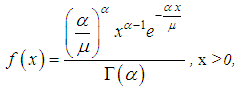 where α is the form parameter (α >0). It is important, that approximate distribution of value of aggregate losing achieved as large as possible probability near zero point. In this situation in actuarial calculations during modelling one can consider gamma- distributions with form parameter for α <0 (see Fig. 1).
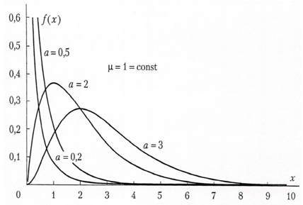 | Figure 1. Probability density of gamma-distribution for different values of form parameter α |
Here Γ (α) is the Euler gamma-function: 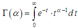 . The gamma-function has the following properties:1) Γ (α +1)=α Γ (α +1) for any positive values для любых α;2) if α is a natural number, than: Γ (α +1)=α !3) Γ (1)=1;
  .The main characteristics of the gamma distribution with parametrization:- average value is equal to M (x)=μ;- dispersion is equal to D (x)=μ2/α;- the coefficient of variation is equal to:
  ;- coefficient of asymmetry is equal to:
  .Estimations of the parameters by the method of moments from the sample data are determine as:
 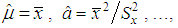 where
where  is the arithmetic average value (sample average value) of losing;
  is the sample dispersion of losing.Now let us the above estimations by the maximum likelihood probability. Gamma-distribution could be considered as a realistic model of aggregate and normalized losses of identically distributed independent risks.Gamma-distribution has an advantageous property: sum of independent gamma- distributed risks has gamma-distribution and in that case, when parameters μi and αi are not equal for all risks. However their relation μi/αi should be constant. In this situation we can model aggregate loss of a group of risks with different insured values by using gamma-distributions.Inverse Gaussian distributionInverse normal (Gaussian) distribution could be used for modelling of non- negative random values. These random values should have more sloping right side of distribution in comparison with left one. At the same time the normal random value could be negative. Framework underwriting during modelling of losing it is usually used inverse Gaussian distribution with parametrization. Framework the parametrization one usually used average value μ of the random value. Probability density of the random value could be written as (see Fig. 2):
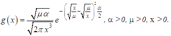 Random value with inverse Gaussian distribution could have positive values only.
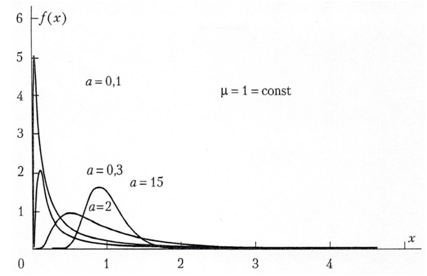 | Figure 2. Probability density of inverse Gaussian distribution |
Parameter μ is the parameter of position, which coincides with average value of random value (as for normal distribution low). Parameter α is the form parameter of the considered probability distribution. Increasing of the parameter α (α →+∞) the inverse normal distribution of probability becomes more like on normal distribution of probability. In this situation framework actuarial calculations (as in the case with gamma-distribution) one can consider α <1.Main characteristics of inverse Gaussian distribution with parametrization:- average value is equal to M (x) =μ;- dispersion is equal to D (x) =μ2/α;- the coefficient of variation is equal to:  ;- coefficient of asymmetry is equal to:
  .Estimations of parameters of moments of random value could be determined as:
 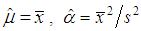 .Inverse Gaussian distribution could be also consider as a realistic model for aggregate and normalized losses framework group of identically distributed independent risks and in many respects similar to the gamma distribution [2].Inverse Gaussian distribution has a property, which coincides with analogous property of gamma-distribution: both distributions will not be changed during using convolution. The property will be saved when parameters αi and μi are not equal for different risks. However relation αi/μi should be constant. In this situation the considered distribution of aggregate lose with different insurance sums.One of advantages of inverse Gaussian distribution in comparison with gamma distribution is the possibility of expressing the distribution function through the standard normal distribution and its tabulated distribution function:
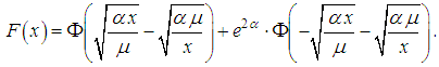 Lognormal distributionContinuous random variable X could be described by logarithmically normal (lognormal) distribution with parameters μ and σ in the case, when the logarithm is subordinate to the normal law and probability density could be written as (see Fig. 3):
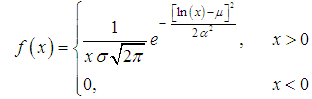
 | Figure 3. Probability density of lognormal distribution |
Logarithmically normal value could be positive only. Because at X >0 inequalities X<x and lnXx are equal to each other, distribution function of lognormal distribution coincides with distribution function of normal distribution of random value lnx: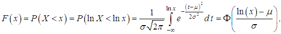 where Φ(t) is the distribution function of standard normal value. The distribution could be written as
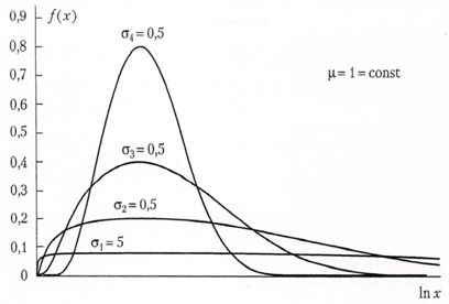
 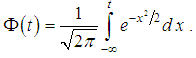 Parameter μ is the scale parameter. The parameter μ is the average meaning of random value framework normal distribution low or median of random value framework lognormal distribution low. As for normal distribution probability density of lognormal distribution can not be integrated to obtain probability distribution function in an explicit form. However values of integral function of lognormal distribution could be determined by using values of the same integral function of standard normal distribution.Lognormal distribution has steep left and sloping right descent, i.e. positive asymmetry. At increasing of parameter μ one can find shifting of probability distribution to right, i.e. come near to normal distribution. Parameter σ is the standard deviation of random value lnx and form parameter. Decreasing of parameter σ leads to increasing of asymmetry of distribution. In this situation framework in actuarial calculations one can use lognormal distribution at small value of σ, when σ <μ.The main quantitative characteristics of the lognormal random quantity are:- average value is equal to
  ;- dispersion is equal to
  ;- the coefficient of variation is equal to
  ;- coefficient of asymmetry is equal to
  .Statistical estimations of parameters μ and σ of lognormal distribution based on sample data could be determined based on moments approach:
  ,
,  . Lognormal distribution could be obtained by multiplication of large number of independent or weakly dependent non-negative random values. Dispersion of every random value should be enough small in comparison with dispersion of lognormal distribution. The logarithmically normal distribution is based on the multiplicative process of the formation of random variables, i.e. framework the process the effect of each additional factor on a random amount is proportional to its achieved level.The lognormal distribution is not invariant with respect to convolution, in contrast to the gamma distribution and the inverse Gaussian distribution, and is well suited for modeling the size of losses in a separate insured event.Collective methods and models of insurance underwritingThe individual insurance underwriting models considered are designed primarily to simulate the average values and variance of the aggregate yearly losing to calculate tariffs. The premise of using these models is the homogeneity of the groups: the risks of each group should be similar in everything, except for insurance amounts.As for the aggregate portfolio of risk insurance policies, it is usually very inhomogeneous, even if it can be divided into homogeneous groups. One of the most important aims of the insurance company is the modeling of the distribution of the loss of the aggregate portfolio. Based on the model of aggregate loss, an idea is constructed about the level of reliability of the company and the required capital. In the collective model of insurance underwriting, it is interesting not only the average value, but also the type of distribution of the aggregate loss. Especially, its right "tail", containing the largest losses, directly determines the level of reliability of the company. Thus, we need a method that allows us to approximate as accurately as possible the aggregate loss distribution of an arbitrary inhomogenous portfolio.The portfolio of risk insurance contracts, as a rule, is very inhomogeneous, so you have to carve up the portfolio into the most homogeneous and independent groups, calculate a loss distribution for them according to the individual model, and then to do convolution of these distributions. However, some groups may be too small, and it is not possible to reliably describe the "tails" of distributions. This problem is typical for risks with high insurance sums, the quantity of which is small, and the influence of the aggregate portfolio on the distribution of the loss is significant.Another, much more successful way was introduced at the beginning of the 20th century by Philippe Lundberg and continued by his compatriot Harald Kramer. The way was finished by the development of a recursive formula that was published in 1980 by Harry Paging and was called the recursive Panger formula [4].The idea of a collective model of insurance underwriting is to consider portfolio only as a producer of losses, not taking into account the belonging of losses to defined risks. This assumption does not lead to losses of information or quality of results, because the initial distributions of the collective model is the distribution of the volume of loss and the distribution of the loss amount-can be estimated much more accurately than the distribution of losses of individual homogeneous risk groups.As in the individual insurance underwriting model, a relatively short period of time is analyzed in the collective insurance underwriting model and it is assumed that the insurance fee is paid in full at the beginning of the analyzed period. However, unlike the individual model, in the collective insurance underwriting model, the entire portfolio of concluded insurance contracts is treated as a single whole, without distinguishing individual contract components. Accordingly, the upcoming insurance events are not associated with certain contracts, but are considered as a result of the company's total risk. It follows that the main characteristic of the portfolio is not the quantity of contracts concluded, but the total quantity of insurance cases for the analyzed period, which is a random variable. Another important difference is that an equal distribution of random variables Yi describing losses due to successive insured events is assumed. This assumption means a certain equivalence of insured events, related to the fact that insurance cases are considered as a consequence of the company's overall risk, rather than individual contracts with their specific characteristics. In addition, random variables Yi describe only real damage and are therefore strictly positive.In collective models it is assumed that the number of insurance cases and losses after the occurrence of insured events are independent in the aggregate. The ruin of the insurance company is also determined by the excess of the total payments Z of the insurer's assets A: ε =P (Z >A); Z=Y1+Y2+…+Yn.In individual models, the average values of payments for each contract are first calculated, and then these averages are summarized by the quantity of contracts. In collective models, the quantity of requirements is modeled, so the summation under contracts is replaced by multiplying two mathematical expectations: M(Z)=M(N)• M(Y).The quantity of insured events in a single contract N is a discrete random variable. Therefore, when modeling the quantity of requirements, discrete laws of distribution of random variables are used. But since qualitatively heterogeneous risks can be contained throughout the portfolio, it is not always possible to use simple, most common discrete distribution laws, often using mixed discrete laws, for example, various mixed (composite) Poisson distributions.Collective models of insurance underwriting for the distribution of the number of insured events. The distribution of the quantity of insured events occurring in one insurance contract during the term of the insurance policy is a discrete random variable that takes integral non-negative values, etc. is the length of the "right tail" essentially depends on the type of insurance. And the longer the right tail of the distribution, the more non-uniform the portfolio is (see Fig. 4).
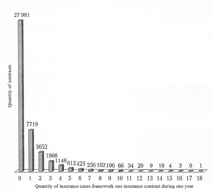 | Figure 4. An example of a histogram of the real distribution of the quantity of insured events in the portfolio of voluntary medical insurance |
The process of data analysis includes the following steps:- processing and grouping of primary information;- estimation of the parameters of the distribution laws of the discrete random variable;- the construction of various theoretical distributions approximating the studied distribution of the number of insured events;- checking of the statistical hypothesis about the form of the distribution law and the distribution parameters;- choosing the best distribution.The classical model of receipt of claims presupposes the following assumptions:- a fixed time interval is analyzed;- the number of contracts n is fixed and it is not random;- the risks are pairwise independent; the occurrence of an insured event under one contract does not affect the occurrence of insured events under other contracts;- treaties are homogeneous, i.e. the likelihood of an insured event p is the same for all contracts.The latter assumption is often broking in practice in real insurance portfolios and for this purpose more complex actuarial models are used in the form of various mixed (composite) distributions. To begin with, consider simple basic distributions suitable for homogeneous portfolios with a small right tail.Poisson distributionPoisson's law is used if the probability of occurrence of an event in each treaty is small, and the number of contracts is large (the law of rare events) and is an approximation of the binomial distribution at n→∞. Insurance cases occur independently of each other with a constant average intensity. The Poisson distribution plays a leading role in modeling the distribution of the quantity of insurance cases, since if it is not used directly, it serves as the basis for constructing mixed Poisson distributions.When modeling the number of insurance cases, the Poisson distribution can be applied to a homogeneous portfolio if several claims can be brought under the contract (not simultaneously), in property, automobile, medical insurance.Discrete random variable is the quantity of insurance claims in a given year or in a separate insurance contract has a Poisson distribution if the probability of occurrence of insured events in one insurance contract is calculated by the relationpk =e-λλk/k!, k =0, 1, 2, …The parameter λ >0 is called as the intensity, it is equal to the quantity of observations of the random variable multiplied by the probability of success in one test: λ =np.Numerical characteristics of the Poisson distribution are: M(K)=D(K) =np =λ. This implies the basic requirement when using the Poisson law: the sample expectation and variance of the number of insurance cases should be approximately equal.The Poisson distribution is the limiting case of a binomial distribution for p→0, n→∞. It follows that the Poisson distribution with the parameter λ =np can be used in place of the binomial distribution, when the quantity of experiments n is sufficiently large, and the probability p is sufficiently small, i.e. in each individual experiment, the interesting event occurs extremely rarely.The statistical estimate of the Poisson distribution parameter  , both by the method of moments and by the maximum likelihood method, from the sample is found as the average value by the following relation:
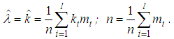 Example 1According to the portfolio of insurance contracts for citizens traveling abroad, in 2016, claims were received in connection with insurance cases for 186 policies out of 29,382. The number of insured events that occurred with one insured person varies from 0 to 2.
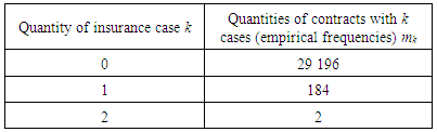
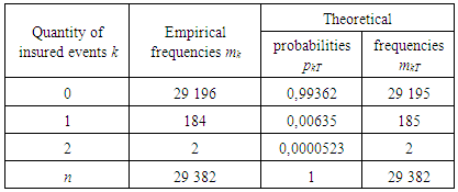
Table 1. Empirical frequencies of the quantity of insured events per insurance policy
 |
| |
|
It is required to simulate the distribution of the number of insured events in one contract with the help of the Poisson distribution and verify its compliance with the Pearson consensus criterion at a significance level of 0.05.SolutionBased on the results of calculations of estimates of the distribution parameters of the random variable k (the quantity of insurance cases in one contract) the following indicators were determined. Selected average value: 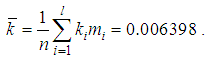 The average quantity of insured events occurring in one insurance contract abroad is 0.0064 for the portfolio under study. Such an extremely low value of the average number of claims, by the way, explains so many low insurance rates for travelers abroad. Selected dispersion:
 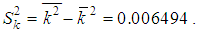 In the portfolio under investigation, the probability of occurrence of the insured event is sufficiently small (m/n=186/29382≈0,0064), therefore for analysis it is possible to apply the Poisson distribution. A statistical estimation of the Poisson distribution parameter has calculated by using the relation:
 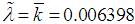 .The results of approximating the quantity of insurance cases for the portfolio of contracts on the basis of the Poisson distribution are given in the table:
Table 2. Results of approximating the quantity of insured events by the portfolio of agreements on the basis of the Poisson distribution
 |
| |
|
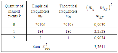
The values of the theoretical probabilities pkT can be calculated by the formula or obtained using the Poisson function (PEASSON (k, ,0)) in MS Excel. Theoretical frequencies are calculated using the Poisson distribution formula: mkT=pkT•n.With Pearson's agreement criterion x2, the adequacy of the model at the significance level σ =0,05 is checked. The results of calculations of the x2 (which were observable) are presented in the following table:
Table 3. Calculation of the statistics of the Pearson criterion for the Poisson distribution
 |
| |
|
Value  . The critical value of statistics can be determined from the distribution tables, or by using the XI20B function in MS Excel. The Poisson distribution has one parameter, estimated from the sample (to combine the intervals did not become so as not to zero the number of degrees of freedom), so
  . In the considered case
  the hypothesis that the number of insurance cases is distributed according to the Poisson distribution is not rejected at the significance level α =0.05, the model is adequate for modeling of the quantity of insurance cases in a given portfolio. It should be noted that the Poisson distribution has come up as a model of the number of insured events occurring in one travel insurance contract (which in practice happens rarely), since the empirical distribution has a very short right tail - the random variable K takes only three values - 0, 1 and 2. And so it turned out that the average and sample variance of the distribution under study are approximately equal. This led to the result.Theoretical distributions used to approximate empirical distributions in collective models of insurance underwriting [5]Negative binomial distributionA random variable K has a negative binomial distribution with parameters (r,p) if in the Bernoulli test sequence with probability of success p and probability of failure q = 1-p, the probability of the number of failures k that occurred prior to the r-th success is determined by the following relation
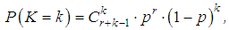 where r is the quantity of successes, positive integer number; k quantity of failures that occurred before the quantity of successes r.Average value and dispersion of a random variable having a negative binomial distribution are equal to:
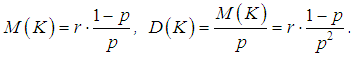 To apply a negative binomial distribution, the dispersion in the quantity of insurance cases must be greater than the average value, so its application in insurance in many cases gives the most adequate result. It is used, for example, in modeling the distribution of the number of insured events of an individual insured for a heterogeneous portfolio of contracts.If the estimation of dispersion from the statistical data is greater than the estimation of the average value, then the moment method can be used to estimate the parameters p and r:
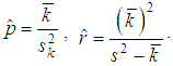 Now we can obtain the limitations on the use of a negative binomial distribution follows: since the probability can not be greater than 1, the average value of the damage should not exceed the dispersion. This situation is very often encountered in practice in inhomogenous portfolios with a long right tail (in insurance LCA, CASCO, etc.), so its application in insurance in many cases gives the most adequate result.Geometric distributionThe discrete random variable K has a geometric distribution with the parameter p if it takes the values 0, 1, 2, ..., k, ... (an infinite but countable set of values) with probabilitiesP(K=k)=pqk.The probabilities P (K = k) represent a geometric progression with the first term p and denominator q, hence the name "geometric distribution".In practice, a random quantity having a geometric distribution is the number of k tests conducted according to the Bernoulli scheme, with probability p of the occurrence of an event in each test, before the first success, i.e., the number of failures before the first positive outcome.The average value and dispersion of a discrete random variable, distributed geometrically, are determined by the formulasM(K)=q/p, D(K)=q/p2.The statistical estimate of the parameter p from the sample is:
 The geometric distribution is a particular case of a negative binomial distribution (for r =1). Therefore, it is applicable when the estimate of the parameter r is close to 1 and the probability p is within acceptable limits.Mixed Poisson distributions for modeling the quantity of insured eventsIn practice, the Poisson distribution parameter λ is often not constant for the following reasons:- the difference between the parameters of the Poisson distribution for different insurers when modeling the number of cases in individual models;- the parameter difference for different years in a portfolio with the same risks in the case of a collective model (weather conditions, economic conditions, etc.). For example, when car insurance against an accident, the intensity depends on the quantity of days with bad weather and is not constant.In this case, the problem arises of introducing an additional random variable Λj that is responsible for changing the parameter λ and reflecting the heterogeneity of the portfolio (in the first case) or serving to model annually changing external impacts in a homogeneous portfolio of the collective model (in the second case). Λj are the independent identically distributed random variables characterizing the insurer's individuality in the first case and the "quality of the year" in the second case. Distribution Λj is called a mixing distribution and acts as a measure of the inhomogeneity of the portfolio. Jean Lemer [6, 7] and Thomas Mack [3] suggest that a certain function called the structure function u (λ), which leads to the so-called mixed (composite, complex) Poisson distribution, should be used to account for the inhomogeneity of policyholders.Suppose that the distribution p(k) (k=0, 1, 2, …) of the number of insured events on the account of each insured person has a Poisson distribution:
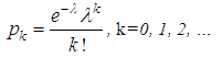 Each insured is characterized by its value λ, which allows to take into account heterogeneity of risks.The discrete random variable K has a mixed Poisson distribution law if it takes the values k=0, 1, 2, …, with the parameter function u (λ) with probabilities:
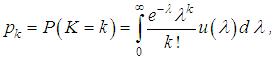 where u (λ) is the distribution density of the random variable Λj (structure function). In practice, a certain assumption is made about the form of the mixing distribution, i.e. distribution of a random variable Λj.As a structural or mixing function, different functions can be selected. The most common as a mixing distribution and result in adequate results:- gamma-distribution;- inverse Gaussian distribution.Mixed Poisson / Gamma distributionAs a Poisson parameter simulating the function in actuarial calculations, a gamma distribution with parameters a and b is often used:
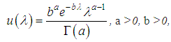 where
where 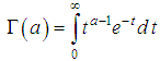 is the Euler gamma function, Γ(a+1)=aΓ(a), Γ(a+1)=a!, a is the natural number. Number characteristics of the distribution are: M(Λ)=a/b; D(Λ)= a/b2. It is the gamma distribution that well describes the situation when the values of λ fluctuate around a certain value, while both very small and very large values of λ are possible, but unlikely. The distribution of the quantity of insured events in the portfolio is {pk, k =0, 1, 2, …} then reduced to the following form:
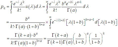 If a is an integer, then, taking into account that Γ(a+1)=a!, one can obtain:
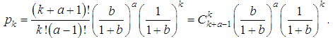 .Thus, we came to a negative binomial model with the form:
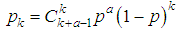 with parameters and numerical characteristics:
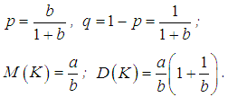 The calculation of the probabilities of a negative binomial distribution does not require a table of values for the gamma function. Consistent use of the property Γ(a+ 1)=aΓ(a) allows us to go over to the recurrence formula:
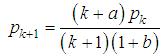 at the initial value
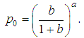 Estimates of the distribution parameters for the sample using the method of moments are carried out by the formulas:
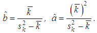 Example 2It is known, that:1) The number of insurance cases K has a Poisson distribution with an average Λ;2) Λ has a gamma distribution with average value 1 and dispersion 2.Let us define probability of that K=1 (in the contract there will be 1 insurance case).SolutionBy the condition of the problem, the random variable K has a mixed Poisson / gamma distribution, which is reduced to a negative binomial distribution of the form:
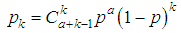 with parameters:p =b/(1+b), q =1-p =1/(1+b),where a and b are the parameters of the gamma distribution that are related to its average value and dispersion by the following relations:M(Λ)=a/b, D(Λ)=a/b2.By condition M(Λ)=1, D(Λ)=2.Hence the parameters of the gamma distribution:
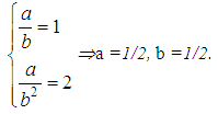 In this situation one can obtainp =b/(1+b)=1/3, q =1-p =1/(1+b)=2/3,Now, using the formula of negative binomial distribution, we can calculate the required probability:
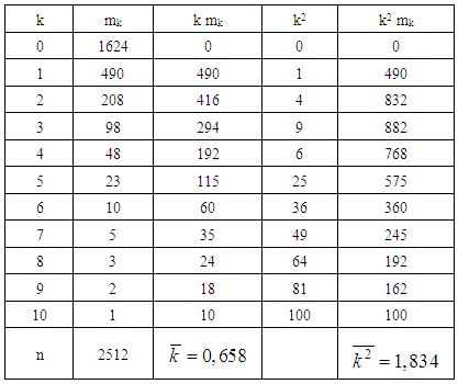
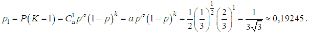 Example 3Let us analyze a portfolio consisting of n =2515 contracts for auto hull insurance. For the year, claims were received for m =888 contracts in connection with insurance cases. Quantity of insurance cases k that occurred under one contract varied in the portfolio from 0 to 10. It is necessary to check whether the mixed Poisson/gamma distribution (negative binomial) is suitable for modeling the distribution of the number of insured events in a given auto hull portfolio.SolutionWe will calculate estimations of the distribution parameters of the quantity of insured events in one contract (average value):
 and selective dispersion
  . The table with results of calculation could be written as:
Table 4. Calculation of sample estimates of the distribution parameters of the quantity of insured events in one contract
 |
| |
|
So, based on the results of calculating the estimates of the distribution parameters of a random variable K (quantity of insurance cases in one contract) we obtain:- sample average: k =0.6584 is in one portfolio contract, an average of 0.658 insured events occur during the year;- sample variance: 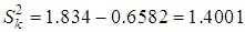 .The verification of this empirical distribution on the Poisson law gave a serious discrepancy between the empirical and theoretical frequencies and
 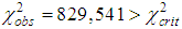 (a=0.05, v=5-2=3)=7.815. Thus, in the example considered, the Poisson distribution can not serve as an adequate model, the empirical distribution has a long right tail (up to 10 insurance cases) it is necessary to try mixed Poisson distributions. So, we calculate the mixed Poisson/gamma distribution.Taking into account the sampling characteristics found, the mean and sample variance k=0.6584,
 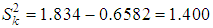 let us calculate estimations of parameters of gamma-distribution:
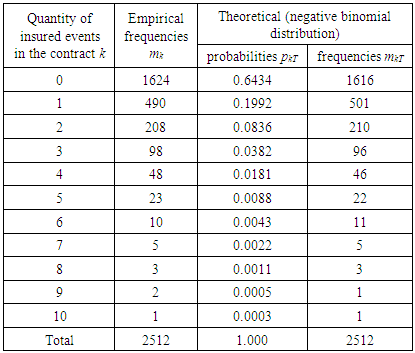
 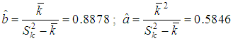 .Using the recurrence formula and the formula for calculating the probability of zero payments, we calculate the theoretical frequencies, the results are presented in the following table:
Table 5. Calculation of the distribution of the number of claims in the portfolio of auto hull contracts using a negative binomial distribution (mixed Poisson / gamma distribution)
 |
| |
|
Further, in accordance with the requirements of the Pearson consensus criterion for combining intervals with small theoretical frequencies less than 5, the observations were grouped together and the value  . Comparison of
  and
and  (a=0.05, v=9-2-1=6)=12.592 shows, that
  . In this situation the verifiable hypothesis is not rejected, i.e. the considered negative binomial model is adequate and assumes as accurately for description of distribution of the quantity of claims. A negative binomial model, adopted at the same level of reliability, can be used for actuarial calculations.Modeling of value of loss in one insurance contract in a collective insurance underwriting model.The collective model assumes that during the time when external factors (in particular, inflation) change insignificantly, the random values of the loss size in a separate insurance event in the portfolio under consideration are independent and equally distributed. If the assumption of independence is recognized as fulfilled, then the assumption of the same distribution seems unrealistic even if in light of the difference in insurance amounts. But, since in a collective insurance underwriting model, losses are not compared with individual risks. However they are considered together in a certain time interval, we can assume that they represent a sample of a single distribution, namely a mixture of different distributions of individual losses.Of course, each type of insurance and each portfolio corresponds to its (mixed) distribution of losses, depending, in particular, on the size of the insured amounts for individual risks, as well as insured events. Thus, the average loss from a fire in an industrial plant is much higher than from a fire in a residential building; both differ from average losses in motor third party liability insurance and motor third party insurance, which in turn differ from each other. But, as practice shows, loss structures in all types of insurance are very similar. Usually, there are many more small losses than large losses. "Concentration of losses" with increasing size of the loss increasingly decreases (it happens, very small losses are also small, but from the economic point of view they do not matter much). However, the quantitative ratio of large and small losses, as well as (in any case, inaccurate) the boundary between large and small losses for different types of insurance is different.For many practical problems, the adequacy of the model of loss size distribution in the field of large losses is most important. In our interests, it is possible to describe more accurately the large loss by the sought-for distribution of the loss size. This most important from an economic point of view, part of the distribution is almost always represented by too few observations. The correctness of modeling the size of the loss in a separate insured event often depends on the correct choice of the appropriate distribution.We list the typical requirements for families of distributions [3]:1. The model should adequately describe the aggregate distribution. Hence, in particular, it follows that the distribution should not allow negative amounts of loss.2. The model should not be too complicated; it is desirable that it contains a small number of parameters.3. The model should correspond to the structure of losses.The most widely used in practice continuous distribution laws used to approximate the distribution of the amount of damage in a single insured event:- lognormal distribution;- logarithmic logistic distribution;- the logarithmic distribution of Laplace;- Pareto distribution with zero point.Let us consider the distributions applicable to modeling the size of the loss. Lognormal distribution is perfectly suited as a model for the amount of loss in a single insured event.Logistic distributionLess well-known, but similar to normal, logistic distribution has a density could be written as:
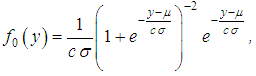 where μ is the average value of losing;
  ; σ2 is the dispersion. Logistic distribution function could be written as:
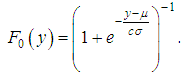 As a result of the transformation x = ey, we obtain the distribution function:
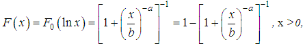 where b=eμ is the scalar parameter; a=1/cσ. The density of the log-logistic distribution is given by
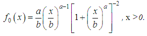 The Laplace distributionThe Laplace distribution with distribution function f (y)=0.5a•e-a |y-μ | is also symmetric and true for all real arguments. The distribution consists of two symmetric relatively μ exponential distributions. The Laplace distribution function could be written as:
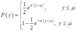 After the transformation x=ey we obtain the logarithmic Laplace distribution b=eμ
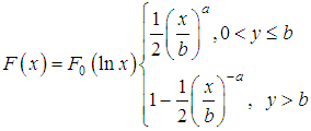 The right-hand side of this distribution after normalization is known as the Pareto distribution. The density of the logarithmic Laplace distribution could be written as
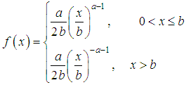 Sites of small and medium losses are not accurately approximated by this distribution, but in the field of large losses the model is acceptable and even slightly overestimates the frequencies.Pareto distributionThe less suitable left-hand part x≤b of the logarithmic Laplace distribution can be replaced by a distribution suitable for describing small losses, for example, gamma or inverse Gaussian distributions. The simplest way to set the Pareto distribution on the interval (0;b) is to shift it to the left by the value b. Then the Pareto distribution with the distribution function:F (x) =1-(x/b)-a, x≥b,is transformed into a Pareto distribution with a zero point with a distribution function:
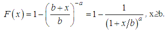 The density of a given distribution is given by the function
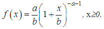 In some types of insurance, the Pareto distribution with a zero point tends to slightly overestimate the frequency of the largest losses. In such cases, one can replace the transformation x =ey by a "weaker" transformation x =yt, t >1. Then the Weibull distribution is obtained from the unbiased exponential distribution with the distribution function F (y)=1-e-β y.Distribution of cumulative damage in collective models of insurance underwriting. The recursive Panger formulaSuppose N is the number of losses of a given portfolio in the time interval of interest (one year), and let X1, X2, ..., XN be independent equally distributed losses. Then the cumulative loss can be represented in the form Z=X1+X2+...+XN. The properties of the conditional mathematical expectation allow us to express the moments of the random variable Z in terms of the moments of the quantities N and Xi:
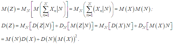 From these formulas it follows that the square of the coefficient of variation is equal to:
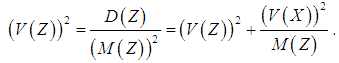 It is much more difficult to obtain the distribution G of the cumulative loss Z. In spite of the central limit law, one can hardly count on the convergence of Z with the increasing of M (N) to the normal value. Experience shows that even large portfolios are asymmetric, and the normal distribution substantially underestimates the probability of a large cumulative loss. Strictly speaking, the central limit theorem is valid only in the case of a Poisson distribution of the number of losses. If N has a mixed Poisson distribution, then the distribution of the quantity Z/M (Z) converges with increasing M (Z) to a mixing distribution (as follows from the formula given earlier for V (Z)).The distribution G of the aggregate loss Z must be obtained from the distributions of the quantities N and X. Unfortunately, there is practically no other way of finding the distribution of the aggregate loss. For a straightforward adjustment of a distribution model, there is almost always not enough data, because every year gives only one observation, and the values of the cumulative loss of distant past years are in most cases not relevant. It is possible to express the distribution of G through the distributions pn=P (N =n) of the number of losses N and the F (x)=P (X <x) distribution of the loss amount X:
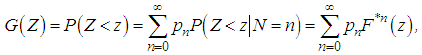 where F*n denotes an n-fold convolution of distributions F(F*0(x)=0 at x<0 и F*0(x)=1 at x≥0).However, an explicit calculation of the infinite sum of the degrees of convolution is possible only in rare unrealistic cases, for example, when N has a geometric distribution (i.e., a negative binomial distribution with parameter r =1), and X is an exponential distribution. A much better approximation of the distribution of Z is achieved by unimodal right-asymmetric continuous distribution models with three parameters (instead of two). The values of the parameters should be determined from the conditions for the equality of the first three empirical moments to the corresponding theoretical moments. After all, the more points coincide, the more similar the distributions themselves are. As the simplest models, biased gamma, lognormal and inverse Gaussian distributions are allowed, with the third parameter in each case giving the zero point offset.The risk theory has generated many other analytical approximations, which in many respects lost their importance today against the background of achievements in the field of numerical approximation. Let's turn to the most popular numerical approximation is the recursive method of Paging. Before applying the method, it is necessary to approximate the distribution function F of the loss size X by an arithmetic discrete distribution
  whose carrier
  takes only the values kh, k =0, 1, 2, ..., K with probabilities fk, where h>0 is the sampling step and f0+f1+…+fk=1. Contrary to the constant requirement X >0, here we purposely admit the value
  , so that when passing from a continuous density to a discrete one, we have an additional probability weight of 0.Although in practice the size of the losses is always presented in a discrete form, it is advisable to first smooth out the imminent randomness (especially in the field of large losses) by continuous density and then again to discretize it. The discrete distribution is most conveniently constructed using the method of equality of local moments. First, from the conditions for the equality of the partial (local) moments
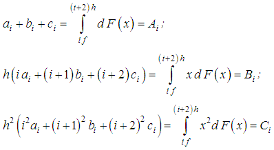 one could determine probabilistic weights ai, bi, ci, i =0, 2, 4, …, K-2 (K is the integer value) for values of losses ih, (i+1)h, (i+2)h. Solving this system with respect to ai, bi, ci leads to the following result:
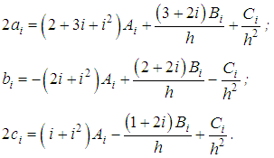 Probabilities fk of discretization
  of distribution F are equal to:
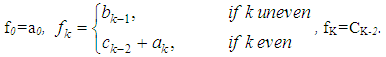 If F has a probability mass to the right of kh (if the support of F takes values up to ∞), it is recommended to add one point z >Kh and distribute the probability A =1-F(K h) as follows:
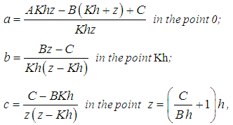 where
where 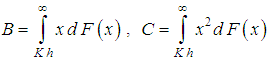 .The inequality z = Kh follows from the condition C> KhB. As a result, the mathematical expectations and variance of distributions
  and F coincide.The aggregate loss
 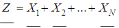 has an arithmetic discrete distribution
  with step h and probabilities
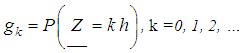 The possibility of specifying a recursive formula for gk depends crucially on the possibility of recursive calculation of the distribution of the quantity N:pn =P(N=n), n =0, 1, 2, …The most common in practice loss distribution distributions are the Poisson distribution and the negative binomial distribution. The are given by the recursive formula:n•pn =(n•a+b) pn-1,where in the case of a Poisson distribution with the parameter λ: a=0, b =λ, and in the case of a negative binomial distribution with parameters a and pa=1-pb=(a-1) (1-p).In the actuarial literature it is proved that only four types of discrete distributions satisfy this recursion. They are binomial, geometric, negative binomial and Poisson. All of them were considered earlier. Now we formulate the recursive formula of the Panger.Let the distribution of the quantity of losses {p|n=0,1,…} satisfy the recursions: npn=(na+b) pn-1, N ≥1. Then the distribution {gk|k=0,1,…} of the total loss, obtained from the arithmetic discrete distribution {fk|k =0,1,…,K; fk=0,k >K} of the loss amount, are calculated using recursive formulas:
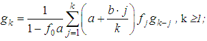
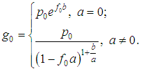 At a large portfolio volume, the value of g0 can be very small, which leads to zeroing of the series. In such cases, transformations of the type a =eln(a) are carried out.
3. Conclusions
In this paper we introduce an analytical approach to model aggregate distribution function of insurance underwriting. Based on the distribution function one can determine possible scathe and profit of financial operations. We compare several approaches of statistical description of financial operations. Based on the comparison we formulate recommendations on using of the distribution functions with comments on positive and negative their properties.
References
| [1] | O.V. Podchishchaeva, and A.V. Dorozhkin, Economics and Enterprise, 83, 1201 (2017). |
| [2] | S. Mori, D. Nakata, and T. Kaneda, Modern Economy, 6, 1001 (2015). |
| [3] | T. Mack, and G. Venter, Insurance: Mathematics and Economics, 26, 101 (2000). |
| [4] | S. Maruthaveeran, “Establishing performance indicators from the user perspective as tools to evaluate the safety aspects of urban parks in Kuala Lumpur”, Pertanika Journal of Social Science and Humanities, 18 (2), 199 (2010). |
| [5] | Y. Kahane, The ASTIN Bulletin, 10, P. 223 -239 (1979). |
| [6] | G.A. Schmidt, M. Kelley, L. Nazarenko, R. Ruedy, G.L. Russell, I. Aleinov, M. Bauer, S.E. Bauer, M.K. Bhat, R. Bleck, V. Canuto, Y.-H. Chen, Ye Cheng, T.L. Clune, A.D. Genio, R. de Fainchtein, G. Faluvegi, J.E. Hansen, R.J. Healy, N.Y. Kiang, D. Koch, A.A. Lacis, A.N. LeGrande, J. Lerner, K.K. Lo, E.E. Matthews, S. Menon, R.L. Miller, V. Oinas, A.O. Oloso, J.P. Perlwitz, M.J. Puma, W.M. Putman, D. Rind, A. Romanou, M. Sato, D.T. Shindell, S. Sun, R.A. Syed, N. Tausnev, K. Tsigaridis, N. Unger, A. Voulgarakis, M.-S. Yao, and J. Zhang, Journal of Advances in Modelling Earth Systems, 6, 141 (2014). |
| [7] | J. Lerner, and J. Tirole, The journal of industrial economics, 50, 197 (2002). |

 Abstract
 Reference
 Full-Text PDF
 Full-text HTML