1. Introduction

As the global population continues to grow, the demand for resources and living spaces escalates accordingly. One critical aspect of resource extraction involves mining facilities, which employ dams to contain the waste generated during the extraction process. This waste material, known as tailings, is composed primarily of fine grains, such as clay, silt and fine sand [1,2]. Tailings are generally transported in liquefied form to the tailing dams through pipeline systems [3]. However, the rheological nature of liquefied mining tailings deviates from the behavior of Newtonian fluids, such as water and oil, being considered a non-Newtonian fluid [4,5]. The study of rheological properties of tailings and their flow plays a vital role in establishing safety protocols and in determining flooded areas for mining waste dams through a tailings dambreak analysis [6]. This analysis is usually carried out with numerical models, which require rheological properties of the flowing material as input parameters. Thus, by investigating the rheological properties of these materials, researchers can establish effective measures to ensure the safety of people living around mining waste dams.

Nevertheless, the study of non-Newtonian fluid flows is a non-trivial challenge, since non-Newtonian rheological models are often more complex than the standard Newtonian model. If the classical Newtonian fluid mechanics theory provides only a few analytical solutions, the non-Newtonian theory provides even less. With the advance of computational power, Computational Fluid Dynamics (CFD) poses itself as a field that facilitates the study of non-Newtonian flows by simulating the behavior of fluids through computational means. By applying numerical methods and algorithms, CFD offers a powerful tool to model and analyze the intricate dynamics of fluids, including the non-Newtonian fluids.

When simulating non-Newtonian fluids, computational dynamics software frequently relies on either the finite difference method or the finite volume method to solve the governing partial differential equations, that ensure a balance of flux, mass, and momentum across the boundaries of discretized control volumes. Noteworthy software used for non-Newtonian fluid simulation includes, for instance, FLO-2D/3D, HEC-RAS, Riverflow2D, DHI MIKE 21/3, FLOW3D, and DAN3D [7].

Within the domain of CFD, Smoothed Particle Hydrodynamics (SPH) has emerged as a paradigm-shifting approach. In contrast to conventional grid-based methods, SPH employs a particle-based framework fit to simulate problems with a complex frontier dynamic. The fundamental principle of SPH revolves around discretising the fluid domain into discrete particles, each with properties like mass, position, and velocity. Interactions between pairs of particles inside smoothing kernels are calculated using hydrodynamics equations that dictate fluid behaviours.

One of the key advantages of SPH lies in its ability to handle fluid flows with high deformability, complex boundaries and free surfaces [8], meanwhile, the treatment of boundary conditions is certainly one of the difficult technical points of the method. The particle-based nature of SPH allows for easier free surface fluid scenarios and handling of multiphase interactions [9], making it well-suited for simulating scenarios such as liquid sloshing [10], dam break simulations, and ocean waves [11]. It also works well with complex and moving boundaries, which are notably difficult to simulate using mesh-based simulations [12].

DualSPHysics was already used to simulate classic dambreak scenarios of non-newtonian fluids and compared to experimental data. A work with non-Newtonian SPH and a real-life dam break scenario was done using an incompressible SPH formulation and achieved good agreement between numerical simulations and available experimental data [13]. Another work with non-Newtonian SPH simulations used a weakly-compressible formulation to achieve numerical results that closely agree with experimental data [14]. These studies exemplify the effectiveness of SPH in capturing the complexities of non-Newtonian fluid dynamics during dam-break events.

However, both of the previously mentioned articles worked with two dimensional simulations of instantaneously released fluid. Studies are missing where three-dimensional unsteady flows are investigated, where the dam break event (breaching) occurs over a certain time period. We overcome that gap by working with a three dimensional simulation, and considering an experiment where a vertical plate represented the dam, which is removed at known speed. Thus, we are taking into account the speed at which the dam rises to mirror experimental conditions. Our hypothesis is that the moving dam boundary could prove to have big influences on the way the fluid behaves throughout the simulations.

Furthermore, as with most numerical approaches, implementing an SPH model to simulate non-Newtonian fluids requires a calibration process to ensure that the simulated behavior accurately reproduces the physical phenomenon of interest. This process involves defining target data that represents the expected model outputs and identifying the parameters to be adjusted. In many cases, calibration is conducted manually through a trial-and-error procedure, where parameters are iteratively tuned until the model results achieve satisfactory agreement with the reference data.

For computationally efficient models, this process can be automated through optimization algorithms such as DSS, which iteratively execute simulations and adjust parameters to minimize discrepancies between simulated and target outcomes. When dealing with more computationally demanding models, however, such approaches become less practical due to the high simulation cost. In these cases, calibration must be approached more strategically, prioritizing simulations that maximize information gain while minimizing computational expense. Such parameter tuning studies are a necessary preliminary step in any computational simulation. However, even though existing for non SPH-based approaches, like Eulerian RANS (Reynolds averaged Navier-Stokes) solvers, such parameter studies have not been undertaken and published so far for SPH models. This knowledge gap will be handled in the presented manuscript, by identifying and evaluating suitable parameters within an SPH-based code with specific emphasis on non-Newtonian fluids, and a dam-break type application case.

1.1. Objectives

The primary objective of this work is to demonstrate the application of the DualSPHysics model to an idealized dam-break scenario involving a non-Newtonian fluid, specifically carbopol gel. We aim to bridge the gap between experimental observations and computational simulations by comparing three-dimensional, unsteady flow SPH-generated results with available experimental data. Secondly we were tuning the model parameters to achieve a closer correspondence between simulation and experiment. The findings presented here are intended to guide future simulations by illustrating how individual parameters influence the behavior of non-Newtonian fluid flows and by highlighting the settings that most effectively reproduce the observed experimental behavior.

2. Rheological Aspects

Rheology can be understood as the science that studies the deformation and flow of materials. In order to characterize rheologically a material, a relationship between shear stress and shear rate is required, producing the flow curve. Several experimental techniques are used to determine the flow curve by exerting a known shear stress and measuring the shear rate, or vice-versa. Then, a rheological model is adjusted to the flow curve points and the corresponding rheological parameters are obtained. The simplest, one dimensional, model is the Newtonian model (equation 1), featuring a linear relationship between shear rate and shear stress, usually denoted as the partial derivative of velocity with respect to a perpendicular direction , and connected by dynamic viscosity .

(1)

Or, in tensorial form:

(2)

where denotes the second-order shear rate tensor and is the second-order strain rate tensor.

Non-Newtonian fluids, however, exhibit a non-linear relationship between shear rate and shear stress. Consequently, a different approach is required compared to the treatment of absolute viscosity. This is where apparent viscosity becomes useful. It is defined as the ratio of shear stress to shear rate , as expressed in equation 3.

(3)

In non-Newtonian fluids, viscosity exhibits a non-linear relationship with shear rate. This behavior can manifest as an increase in viscosity with increasing shear rate (shear-thickening) or a decrease in viscosity with increasing shear rate (shear-thinning). Beyond these variations in viscosity, another defining characteristic of non-Newtonian fluids is their response to shear stress. In certain conditions, the fluid may behave like a solid, resisting deformation and showing no flow until the applied shear stress exceeds a critical threshold.

To account for the effects of the non-linear relationship between shear rate and shear stress, the non-Newtonian general model is employed (equation 4). In this model, the shear stress tensor is dependent on the strain rate tensor (D) in a non- linear manner, which implies that the viscosity is a function of the shear rate. The strain rate tensor, also referred to as the rate of deformation tensor, describes the rate at which fluid elements deform.

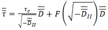(4)

In this equation, is a characteristic stress parameter that represents the stress contribution in the first term of the model. The term denotes the second invariant of the strain rate tensor.

The power-law model, for example:

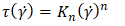(5)

In tensorial form:

(6)

is able to model shear-thinning or thickening properties, where the shear stress is not directly proportional to the shear rate. Shear-thinning fluids, also known as pseudoplastic fluids (n < 1), such as certain polymer solutions, display a decrease in apparent viscosity as the applied shear rate increases. On the other hand, shear-thickening fluids, also known as dilatant fluids (n > 1), such as suspensions of cornstarch in water, exhibit an increase in apparent viscosity with increasing shear rate. The Newtonian model is recovered if n = 1. In this model, the dynamic viscosity is replaced by the consistency .

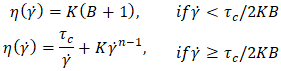
In the context of liquefied mining tailings, these materials are commonly described as viscoplastic fluids, or yield stress fluids [15]. They require a certain amount of stress, known as the yield stress (τc), to start deforming. For an applied shear stress below the yield stress, the fluid behaves as a solid material, resisting deformation. Once the yield stress is overcome, flow starts, and the fluid exhibits liquid behavior. A more general rheological model, the Herschel-Bulkley model [16], captures both shear-thinning (or dilatancy) and viscoplasticity, as shown in Equation 7:

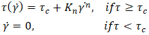(7)

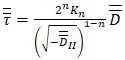
with the shear stress represented as . If and the Bingham model is obtained, which is commonly employed to describe liquefied tailings [3]. As the DualSPHysics code utilizes rheological equations in a one-dimensional format, this and subsequent equations are exclusively expressed in a one-dimensional manner.

The application of rheological models in CFD relies on including them at the viscous term of the governing momentum equations. Equation 8 shows the Herschel-Bulkley model in terms of apparent viscosity η, by dividing Equation 7 by .

(8)

If the shear rate approaches zero, particularly in regions where the flow is nearly uniform, the apparent viscosity tends to infinity. This phenomenon leads to numerical instabilities in numerical simulations. Consequently, regularization models are employed to address this challenge, with various methods being explored in the literature. One notable approach is the Herschel-Bulkley-Papanastasiou model [17] (equation 9 below). Another approach is bi-viscosity models [18].

(9)

With the equation above having the same variables as the equation 8, but with an added exponential term with a calibration parameter m to account for the discontinuity, the model’s behaviour will approach that of the Herschel-Bulkley model in equation 8 as the argument of the exponential increases.

In this study a Bingham model is employed with a regularization parameter B to tune the yield region and keep the apparent viscosity from becoming too high:

(10)

This equation keeps the behaviour of the fluid consistent with the Herschel-Bulkley model for higher strain rates and prevents the apparent viscosity from reaching high numbers at lower strain rates.

3. SPH Background and Formulation

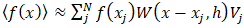
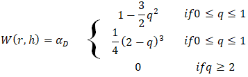
The Smoothed Particle Hydrodynamics (SPH) method was originally introduced by Gingold & Monaghan in 1977 as a computational technique for simulating astronomical phenomena. It’s formulated (equation 11) as the convolution of a function and a kernel function, , with h being the smoothing length of the kernel function, on a point x over an domain [19]. The kernel function plays a crucial role in SPH by approximating the behavior of a Dirac delta function, facilitating the smooth spread of properties and interactions between neighbouring particles.

(11)

Upon employing the equation (11) across the spatial domain, where f denotes a property of interest within the domain, the continuous medium undergoes a process of discretization. In this discretised representation, the continuous domain is subdivided into individual particles. Each particle represents specific attributes of the underlying continuous domain in a discrete form. This discretization process allows us to transition from a continuum representation to a particle-based representation. Once this transition is made, the properties of each particle need to be updated throughout the simulation and the interactions between particles must be calculated. To achieve this, we discretise the equation into a finite form:

(12)

considering all neighbouring particles (j) within the smoothing length of the kernel and their pairwise interaction with the particle to be updated (i). By considering these neighbouring particles, we can accurately update the properties defined by the function f(x) and account for the influences of nearby particles. A visual representation of the updated particle and the support kernel containing the neighbouring particles that influence each update is in figure 1.

Figure 1. SPH particles and Smoothing Kernel Representation

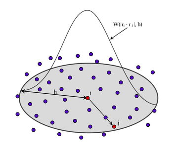
By making i our interpolation particle and j the support particles, writing as meaning the value of the kernel function between the two particles and considering the volume as the ratio between the mass and the density of the particle j, we can rewrite the SPH interpolation as:

(13)

In order to emulate the functionality of the Dirac delta function, the smoothing kernel employed in SPH simulations must adhere to specific conditions. Firstly, like the Dirac delta function, the integral of the kernel function over the domain must equal one. This ensures that the integral of the kernel remains bounded between zero and one, preserving the conservation properties of the simulation. Additionally, the kernel function must exhibit sufficient smoothness to allow the computation of derivatives [20].

As we study fluid dynamics, we need to use the SPH discretization on key equations that govern fluid behaviours. These equations include the Cauchy momentum equation and the continuity equation. With these equations we aim to solve and find velocity, pressure and density. With three variables to solve for and two equations, there is a need for a closing equation. The one implemented in DualSPHysics was proposed as a closing equation for SPH models [21].

4. Methodology

The SPH DualSPHysics model was employed to simulate a scenario akin to experiments conducted on non-Newtonian Carbopol gel [22]. Various configurations of the DualSPHysics model were evaluated to determine the optimal setup for achieving improved accuracy in comparison to experimental data.

While applying the DualSPHysics model, its effectiveness hinges not only on choosing the right parameters but also ensuring its fine-tuning through calibration. This relationship between parameter sensitivity and model fit determines the accuracy with which the simulation mirrors experimental data. In this study, we delve into the process of calibration, aiming to optimize parameters and elevate the model’s fidelity to real-world observations.

However, not all settings prove equally effective. Through this work, we identify and separate configurations that do not yield satisfactory results. This preliminary step is crucial before comparing various combinations of settings that result in more subtle differences between each other, ensuring a more concise analysis. The configurations tested and compared in this work are shown in the flowchart (Figure 2). The ones that were shown to be worse are not taken through to the final scenarios tested.

Figure 2. Flowchart of the Scenarios Simulated Throughout this work

Our initial simulations utilized a specific configuration chosen for its proximity to the final, optimized setup presented later in this article. This setup employed a Verlet time step, Wendland smoothing kernel, Laminar and sub-particle turbulence approximation viscosity treatment, Fourtakas particle shifting, and the SPH method for calculating fluid shear strain. This selection offered a starting point for assessing the sensitivity of our results to other settings and understanding their influence on deviation from expected, experimentally validated outcomes.

4.1. Experimental Scenario

A typical dambreak experiment was set up using Carbopol gel and a camera to record how the fluid flows [22] (figure 3). The dam was represented by a vertical plate. The dam break was simulated by rising the plate at a steady rate to keep the velocity constant. The fluid’s reach was taken from the images recorded with the camera and applying the Canny Edge Detector algorithm [23]. Data compared was from a scenario with rising dam speed of 0.17 m/s. Two sensor were also mounted on top of the experiment to measure the fluid depth by measuring the distance from the sensor to the fluid. One sensor 615 mm from the back of the tank and the second 725 mm from the back. Initial setup parameters scheme can be seen in figure 4.

Figure 3. Experimental Tank Initial Setup for Data Recording from [22]

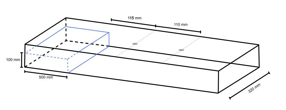Figure 4. Experiment and Simulation Starting Configuration and Dimensions

The fluid’s rheological properties were defined using a rheometer and determining Herschel-Bulkley coefficients: shear yield stress , consistency and flow index (n) [24]. A gel solution of Carbopol 996 polymer with 0.17% mass was used. Its adjusted properties are density of 1000kg/m³ and rheological properties: 57.12 Pa shear yield stress, 15.35 consistency and 0.420 flow index.

The non-Newtonian characteristics and parameters were incorporated into the DualSPHysics model. Meanwhile, the experimental geometry served as the model’s initial condition, providing a foundation for attempting to replicate the observed results.

4.2. DualSPHysics

This work was made using the open-source DualSPHysics model [25], which uses both the computer’s CPU and GPU for processing, making it more efficient and faster than a regular CPU implementation due to the architecture difference. The GPU implementation of SPH via CUDA benefits from the inherent centered and explicit nature of the formulation [26].

CUDA serves as a powerful programming platform facilitating the utilization of a computer’s Graphics Processing Unit (GPU) for general-purpose computing. Harnessing the distinctive architecture of GPUs, it enables superior computing performance in tasks demanding a high level of parallelization. This stands in contrast to computations executed solely by the computer’s Central Processing Unit (CPU), as the GPU’s architecture excels in parallel processing [27].

With this approach, the properties of each particle can be updated independently during each time step. This characteristic allows for efficient parallelization, enabling the simultaneous update of multiple particles as long as there is sufficient computational power available. By harnessing the capabilities of GPU processing, the SPH implementation becomes highly optimized, enhancing the speed and efficiency of the simulation [28].

The model setup steps are outlined in the following flowchart (Figure 5). It’s important to note the sequence of setup steps, as the initial and boundary conditions depend on the smoothing length due to the potential gap formation between boundaries and fluid particles, which is further explained later. Post-processing is configured separately in DualSPHysics, as desired variables need to be calculated using the SPH summation formula (equation 12) for each desired position that isn’t occupied by a particle.

Figure 5. Flowchart of the Setup Steps used for running DualSPHysics model

4.3. Initial and Boundary Conditions

As mentioned earlier, the initial conditions for the SPH model are configured based on the experiment’s geometry. The conversion of the experiment’s physical components, including walls and the fluid, into discrete particles is achieved by implementing SPH equations with an internal particle distance set at 0.004 m. The boundary particles and the rising dam can be seen in figure 6.

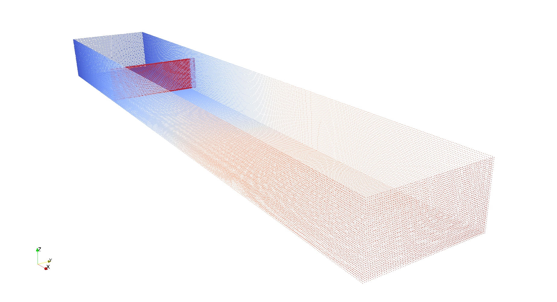Figure 6. Boundary Particles Used on the SPH Simulations

Boundary conditions in the SPH model are established by configuring particles that remain stationary. However, these stationary particles undergo updates in their density throughout the simulation, mirroring the behavior of other SPH particles [12]. This continual adjustment in density serves as a mechanism that prevents particles from breaching the simulation borders, as opposed to a simple no-slip condition [29].

In order to simulate the ascending plate (dam removal), a specific set of boundary particles constituting the dam are given a consistent upward velocity of 0.17 m/s. Different from the stationary particles used in typical boundary conditions, these particles had a fixed non-zero speed.

4.4. Resolution and Particle Density

When employing SPH, there’s no need for a grid that must be refined locally and tailored to the desired domain. Also, unlike traditional numerical methods like finite differences, SPH doesn’t follow the same convergence conditions. Therefore, determining the resolution must be approached differently.

What is commonly employed to determine the particle density in SPH simulations is doubling the number of particles modelled until the results converge between two simulations [30,31]. This way ensures the particle number is no longer affecting the simulation by means of lack of particles or by a saturation of particles inside the smoothing length [32].

The resolution employed in this work was of 0.004m between each particle, resulting in a total of 305,077 particles. While this resolution fits the previously mentioned criteria (half of this resolution wields the same results), it was chosen as to use all the computational power available, as our used machine couldn’t handle higher resolutions.

The computer used for the simulations had an Intel i5 10th generation processor (model i5-10400F) with 16 gigabytes of available RAM and a NVIDIA GeForce GTX1650 with 4 gigabytes of dedicated GPU memory that was used for the simulations.

4.5. Bi-Viscous Calibration Parameter

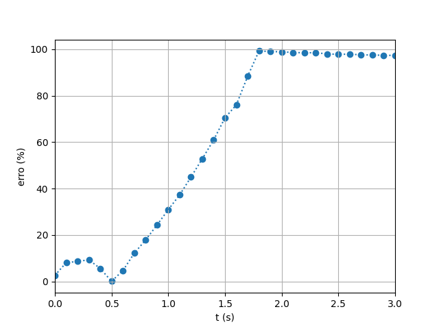
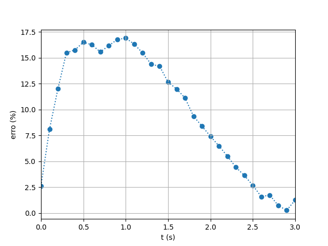
As mentioned earlier, the utilization of the bi-viscous formula involves a calibration parameter. To determine the optimal value for this parameter, a series of simulations were conducted, each employing different values for the calibration parameter. The average relative error was calculated for each calibration parameter simulation in order to find the lowest relative error. The objective was to discern which parameter value would most closely simulate the previous experimental outcomes.

The outcomes of these simulations are visually represented in figure 7 showing the position of the head of the flood wave versus time. The best fit was chosen based on the lower average relative error in relation to the experimental data, the values for the average relative error are shown in figure 8. The value of B=0.005 exhibits a commendable level of agreement with the lowest average relative error of the other simulations of 10%. However, it is imperative to note that, particularly during the initial phases of the flow, the simulation does not entirely align with the experimental data.

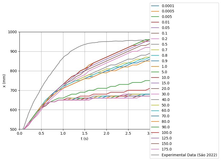Figure 7. Simulation Results for the position of the head of the flood wave versus time for each tested non-Newtonian Calibration Parameter

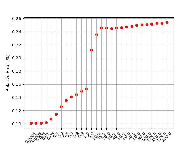Figure 8. Average Relative Error for Each Tested Calibration Parameter

4.6. Shear Rate Calculation

In DualSPHysics, shear rate can be calculated through two different ways. The first employs the conventional Smoothed Particle Hydrodynamics (SPH) formulation to obtain velocity derivatives. The second method involves an adaptation of Finite Differences (FDA), determined by the difference between the velocity of a particle and that of its neighboring particles.

4.6.1. SPH Calculation for Shear Rate

A fundamental expression for calculating the derivative of a function within Smoothed Particle Hydrodynamics [33], is given by:

(14)

Here, ∇f represents the derivative of the function, and ∇W signifies the derivative of the smoothing kernel. This formulation allows us to obtain derivatives by utilizing solely the derivative of the kernel. In the context of calculating shear rate, velocity is employed to determine the rate concerning the direction perpendicular to the line connecting the particles.

The outcomes of the simulation utilizing the SPH calculation for shear rate are depicted in Figures 9 and 10. Notably, these figures correspond to the identical settings employed in the earlier determination of parameter B. Figure 11 shows the evolution of the relative error between simulated and experimental measurements. The average relative error for the flow reach was approximately 10%, while comparisons with Sensors 1 and 2 presented errors of 12% and 23%, respectively. These values indicate a generally good level of agreement, particularly considering the strong non-Newtonian behavior of carbopol gel. The SPH formulation therefore proved capable of reproducing both the overall flow front progression and the local depth evolution with reasonable accuracy.

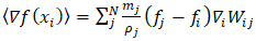
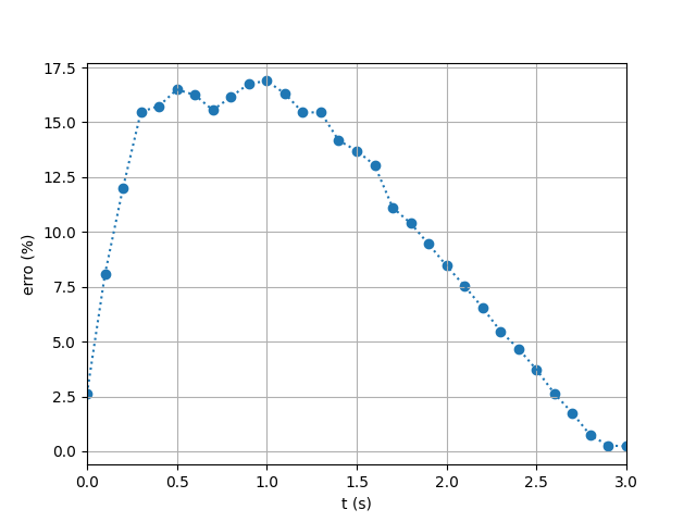
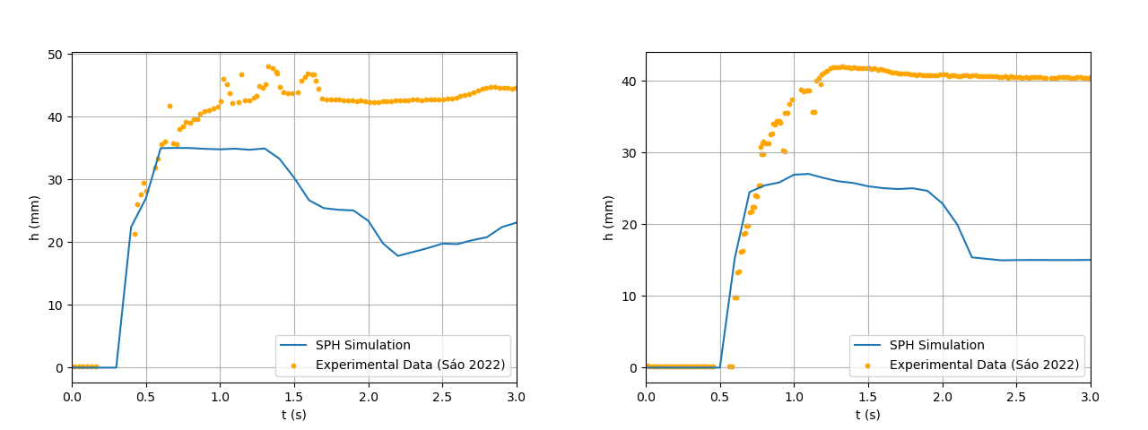
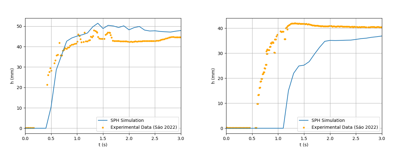
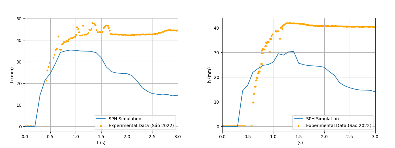
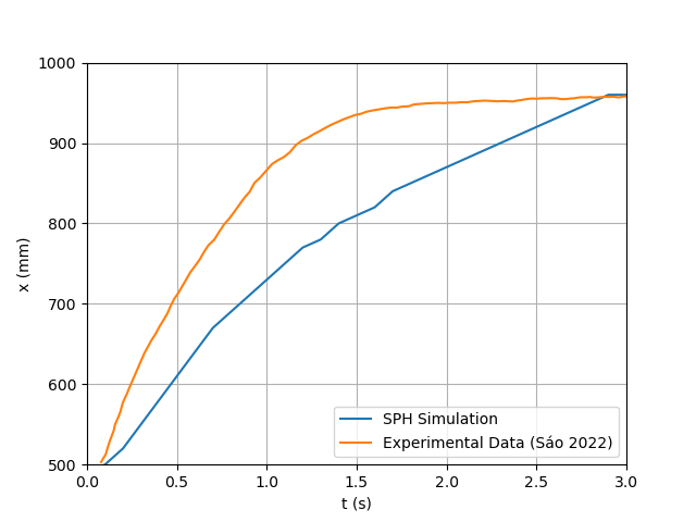
Figure 9. SPH Results for the Dambreak Wave front Reach Throughout the Simulation Using SPH Shear Rate Calculation

Figure 10. Figure 10: SPH Results for Depth Below each Sensor (1 on the left and 2 on the right) Throughout the Simulation Using SPH ShearRate Calculation

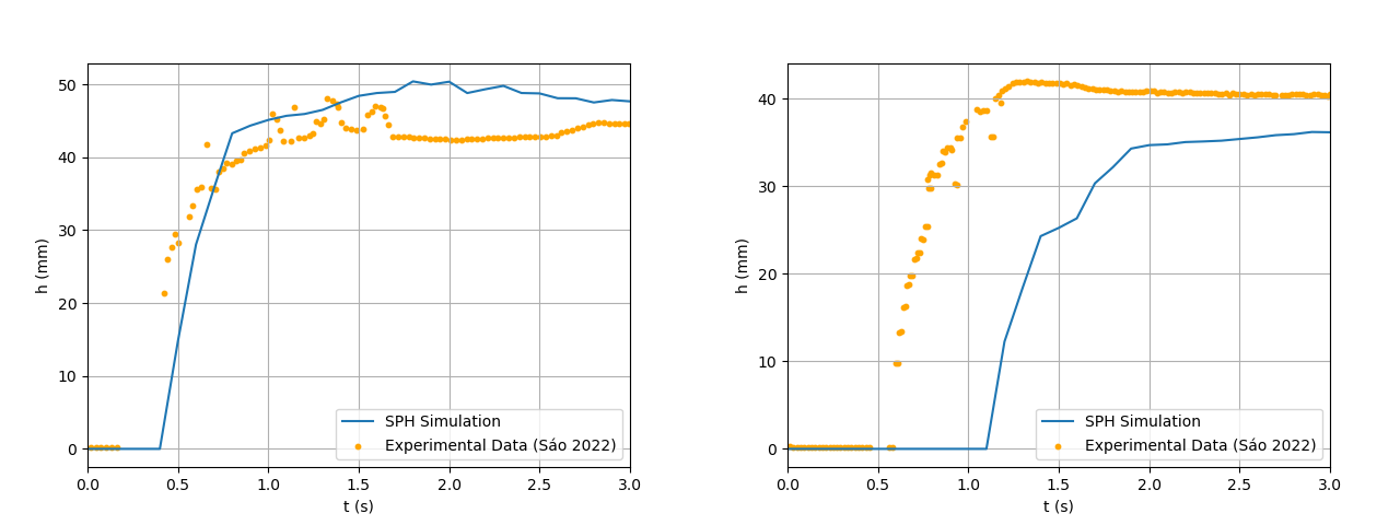
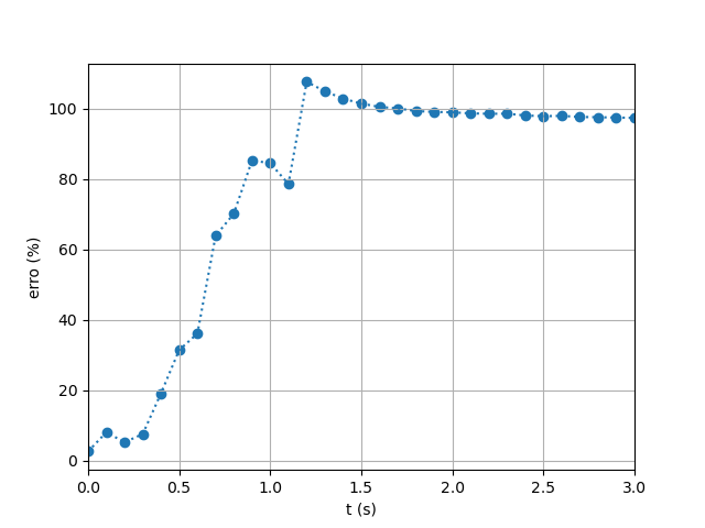
Figure 11. Relative Error Throughout the Simulation for SPH Calculation of the Shear Rate

4.6.2. SPH Calculation for Shear Rate

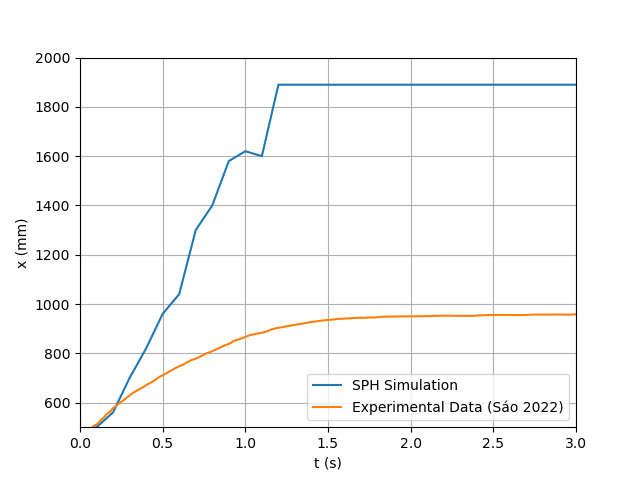
In contrast to the SPH formulation, the FDA method employs finite differences between particles to compute shear rate. This approach is comparatively simpler to implement than the SPH method.

Figures 12 and 13 show the simulated flow reach and depth beneath each sensor using the FDA approach. The corresponding relative errors (Figure 14) were considerably higher on average: 59% for the reach, and 36% and 44% for Sensors 1 and 2, respectively. These deviations suggest that the FDA method was unable to adequately reproduce the fluid’s rheological behavior, leading to poorer agreement with experimental data.

Figure 12. SPH Results for the Dambreak Wave Reach Throughout the Simulation Using FDA Shear Rate Calculation

Figure 13. SPH Results for Depth Below each Sensor (1 on the left and 2 on the right) Throughout the Simulation Using FDA ShearRate Calculation

Figure 14. Relative Error Throughout the Simulation for FDA Calculation of the Shear Rate

The comparison between the two approaches highlights the importance of an accurate shear-rate evaluation in simulating non-Newtonian flows. The SPH formulation, by consistently accounting for particle interactions through the kernel gradient, captured the fluid’s response more realistically and provided superior stability and accuracy. In contrast, the FDA method introduced excessive numerical noise and failed to represent the viscosity-dependent deformation correctly. Consequently, the SPH-based approach was adopted for the remaining analyses in this study, as it offers a more reliable framework for modeling shear-dependent viscosity in non-Newtonian dam-break scenarios.

4.7. Kernel

Selecting the most suitable kernel is crucial for an effective simulation. Polynomial expressions are often favored for their computational efficiency. In our comparison, we evaluate the performance of both cubic and quintic formulations, the former being developed by Monaghan & Lattanzio and the latter by Wendland.

4.7.1. Cubic Spline

The kernel cubic spline formulation [20] is expressed as:

(15)

Here, the variable denotes the distance between particles, and the coefficient is set to for the three-dimensional kernel. The simulation results are presented in Figures 15 and 16 and the error evolution is presented in figure 17. The average relative errors for this simulation’s flow reach were 10% and the sensors presented errors of 13% and 22%, respectively, which indicates a good level of agreement between simulated and experimental data.

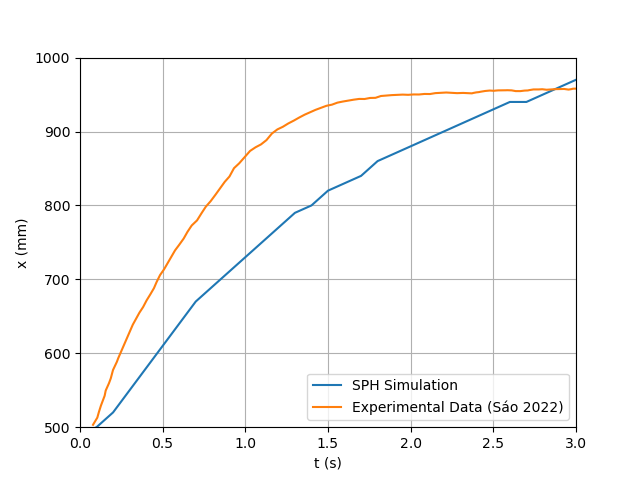Figure 15. SPH Results for the Dambreak Wave Reach Throughout the Simulation Using Cubic Kernel

Figure 16. SPH Results for Depth Below each Sensor (1 on the left and 2 on the right) Throughout the Simulation Using Cubic Kernel

Figure 17. Relative Error Throughout the Simulation for Cubic Spline Kernel

4.7.2. Wendland

In this case, the smoothing kernel employed is a quintic equation [34]:

(16)

where q represents the distance between two particles and the coefficient is set to for the three-dimensional kernel. This also being a polynomial equation means it will also benefit from reduced run times.

The simulation results and comparison to experimental data are shown in figures 18 and 19 and the The relative error calculated for the simulation results using the Wendland kernel are shown in Figure 20. The average relative error was 10% for the reach and 12% and 23% for each sensor, which shows a good level of agreement between simulated and experimental data, just as the cubic spline kernel.

Figure 18. SPH Results for the Dambreak Wave Reach Throughout the Simulation Using Wendland Kernel

Figure 19. SPH Results for Depth Below each Sensor (1 on the left and 2 on the right) Throughout the Simulation Using Wendland Kernel

Figure 20. Relative Error Throughout the Simulation for Wendland Kernel

Upon comparing the results, it’s not obvious which kernel formulation performed better than the other. The differences in average relative error are also very small, being Cubic Spline better by 1% on the first sensor and the Wendland kernel better by 1% also on the second sensor’s results. Since these differences are very minor and within the uncertainty range of the experimental data, it indicates that both kernels are capable of accurately reproducing the rheological behavior of the Carbopol gel.

The Wendland kernel was selected, in the end, for further simulations, because its simulation results did not go over the maximum reach measured experimentally, while the Cubic Spline results did, suggesting a more physically consistent damping of particle interactions near the wave front.

4.8. Artificial Viscosity

Artificial viscosity serves as a crucial technique in SPH formulations to mitigate shock discontinuities. Its primary function is to eliminate gaps between particles, thereby reducing inter-particle penetration and enhancing the simulation’s resemblance to a continuous domain of fluid [35].

In this study, we assessed the effectiveness of two viscosity schemes. The first is a widely adopted approach [35], while the second involves a more sophisticated combination of laminar viscosity and sub-particle turbulence introduced by [11].

4.8.1. Using Artificial Viscosity

The outcomes of employing standard artificial viscosity are depicted in Figures 21 and 22. This approach was originally designed for Newtonian flows and shock-dominated regimes, and it proved inadequate for representing the yield-stress behavior of the Carbopol gel used in the experiments. Notably, it fails to adequately produce the expected deacceleration as the fluid flows, resulting in a deviation from the experimental results.

The artificial viscosity’s employment’s failure to capture the rheological properties is further enforced by the calculation of the relative errors, as shown in Figure 23 for the dambreak reach. The average relative error throughout the simulation was of 77% for the dambreak reach and of 39% and 64% for depth below the first and second sensors. Such high discrepancies reveal that the artificial viscosity formulation distorts the flow dynamics and cannot be relied upon for accurate representation of non-Newtonian fluids.

Figure 21. SPH Results for the Dambreak Wave Reach Throughout the Simulation Using Artificial Viscosity

Figure 22. SPH Results for Depth Below each Sensor (1 on the left and 2 on the right) Throughout the Simulation Using Artificial Viscosity

Figure 23. Relative Error Throughout the Simulation Using Artificial Viscosity

4.8.2. Laminar Viscosity and Sub-Particle Turbulence

In contrast, the scheme employing laminar viscosity and sub-particle turbulence, showcased in Figures 24 and 25, more accurately reproduces the rheological properties of the fluid. The relative error calculated for the simulation results using the laminar and sub- particle turbulence artificial viscosity scheme are shown in Figure 26. The average relative error was 10% for the reach and 12% and 23% for sensor 1 and 2, respectively.This method introduces an explicit laminar term that captures the base viscous resistance of the fluid while the sub-particle turbulence component accounts for unresolved small-scale turbulence. Together, they allow a more realistic representation of the internal energy dissipation mechanisms in yield-stress materials.

The corresponding relative errors (Figure 26) further support this conclusion. The average relative error for the wave reach was 10%, and 12% and 23% for sensors 1 and 2, respectively, a dramatic improvement over the standard formulation.

Figure 24. SPH Results for the Dambreak Wave Reach Throughout the Simulation Using Laminar and Sub Particle Turbulence

Figure 25. SPH Results for Depth Below each Sensor (1 on the left and 2 on the right) Throughout the Simulation Using Laminar and Sub Particle Turbulence

Figure 26. Relative Error Throughout the Simulation Using Laminar and Sub Particle Turbulence

These results demonstrate that laminar viscosity with sub-particle turbulence model more accurately reproduces the rheological properties and momentum dissipation of the Carbopol gel, particularly during the deacceleration phase of the dam-break. Consequently, this formulation was adopted for all subsequent simulations, ensuring both numerical stability and physical fidelity.

4.9. Remaining Scenarios

Three options for artificial density diffusion and two choices for time-stepping schemes were considered with the lack of a clear best choice among the individual options, we opted for a comparison of all six possible combinations. This approach allowed us to delve deeper than individual evaluations and look for subtle improvements visible due to the combination of these parameters.

4.9.1. Time-Stepping

As with other computational fluid dynamics models, the time-stepping scheme plays a crucial role in maintaining stability and ensuring convergence of the Smoothed Particle Hydrodynamics model. While explicit solvers are popular due to their computational efficiency, they can be susceptible to instabilities.

As a first approach, we explored the Verlet time-stepping scheme introduced by [36]. Its popularity in particle dynamics stems from its computational efficiency, making it attractive for large SPH simulations. The Verlet scheme updates particle positions, velocities, and densities at each time step. However, due to the decoupling of the density equation in SPH, an intermediate time-step is necessary for updating density before advancing positions and velocities. This additional step slightly increases the computational cost compared to a fully Verlet-compatible density update, but it maintains stability and accuracy in SPH simulations.

We also investigated a hybrid symplectic-Verlet time-stepping scheme. This approach combines the stability and energy-preserving properties of symplectic integration with the computational efficiency of the Verlet scheme for certain variables. This scheme follows the formulation proposed in Ref. [37], applying symplectic integration to update particle velocities and positions. Meanwhile, the formulation proposed for density calculations in Ref. [38] is also adopted.

4.9.2. Density Diffusion

To mitigate density fluctuations and reduce noise caused by shocks and turbulent flows an artificial density diffusion scheme was introduced [39]. This approach evens out density values among neighboring particles, promoting a smoother density distribution throughout the computational domain.

Beyond the original formulation [39], we test one other way to calculate the density diffusion and the model without density diffusion for comparison. The second formulation tested was proposed in Ref. [40], by Fourtakas et al., in a way to improve the behaviour of particle’s density values close to boundaries.

5. Results and Discussion

The results for the dam break reach for combinations of the time stepping and density diffusion are shown in Figure 27 while the depth below the sensors are compared in Figure 28 for the first sensor, and in Figure 29 for the second one.

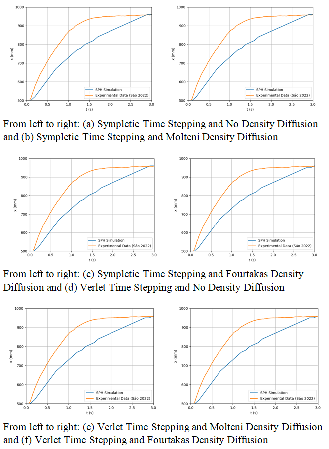Figure 27. From (a) to (f), SPH Results for the Dambreak Wave Reach Throughout the Simulation For the Remaining Scenarios

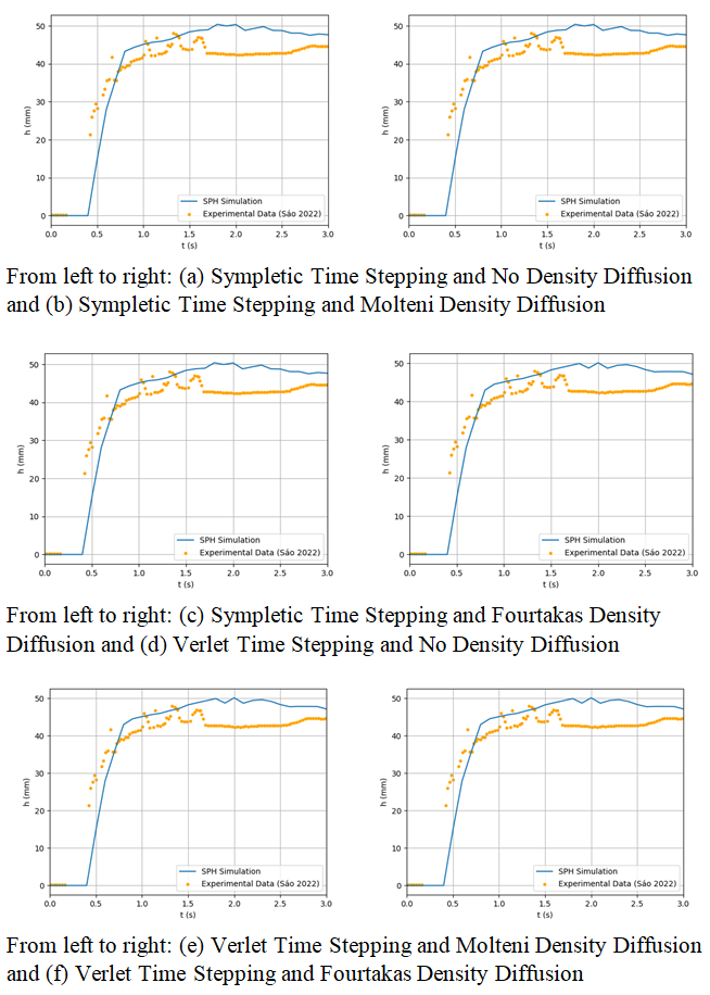Figure 28. From (a) to (f), SPH Results for Depth Below the First Sensor Throughout the Simulation for The Remaining Scenarios

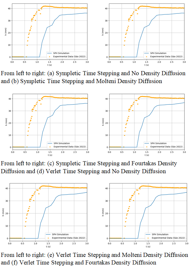Figure 29. From (a) to (f), SPH Results for Depth Below the Second Sensor Throughout the Simulation for The Remaining Scenarios

A comparative analysis indicates that no single configuration outperformed the others. Instead, the differences were marginal, suggesting that within the tested parameter ranges, both the time-stepping and density diffusion schemes provide similarly reliable performance for this type of non-Newtonian dam-break scenario.

By looking back at the settings compared, we can trace how the optimal configuration for the simulations was determined. In several cases, such as the kernel options and viscosity formulations, a superior option emerged. However, for the time-stepping and artificial density diffusion the results show no clear better option.

By comparing the average relative error throughout the simulations across all simulations, we can select a better option by a marginal difference. The density diffusion different methods don’t result in any difference in the results; this suggests big enough density gradients don’t occur during the dambreak simulations for the density diffusion to be meaningful. Thus, for this type of flow, the inclusion of artificial density diffusion does not appear to improve numerical accuracy.

In contrast, a small yet measurable difference was observed between time-stepping schemes. The Sympletic time-stepping average relative errors were of 10% for the dambreak wave reach, 12% for the depth below the first sensor and 24% for the depth below the second sensor. Meanwhile, the Verlet time-stepping average relative errors were of 10% for the dambreak wave reach, 12% for the depth below the first sensor and 23% for the depth below the second sensor. Although these differences are small, this means that using the Verlet time stepping had a better match to experimental data, suggesting an improvement in temporal consistency for this setup.

Overall, these findings suggest that both time-stepping schemes perform comparably well for non-Newtonian dam-breaks under tested conditions, while the density diffusion scheme had no influence on the simulation outcomes, Because of this, the Verlet time-stepping without artificial density diffusion was the selected configuration for this particular scenario, as it offers the best balance between numerical accuracy and computational efficiency.

6. Conclusions

The adjusted non-Newtonian formulation appeared to closely mimic the behavior of the original Herschhel-Bulkley model. Since the objective was to help the lower deformation stages of the flow not to deal with too high apparent viscosities, the formulation used was proven to be suitable for its use.

Ultimately, we couldn’t properly adjust the model simulation to fit the experimental data. While certain aspects exhibited agreement between the simulated and the mea- sured, notably the middle section of the dam-break flow and the fluid depth measured below both sensors, it was not enough to fit the entire simulated results to experimental data.

Since most of the disparity occurred in the early to middle parts of the simulation, the way the moving dam was implemented might be the source of the disparity. As previously mentioned, the boundary particles interact with the fluid particles by increasing density around them and preventing fluid particles from crossing. The gap they might form around that was accounted for during the boundary setup might not work properly around the moving dam, causing repulsion between boundary and fluid when there shouldn’t be, especially below the dam while it rises. This may prevent the fluid from flowing when it should flow, during the first time steps, and constrain flow in a way it shouldn’t, during the middle steps of the simulation. As the dam stops influencing the flow, it matches the experimental data better in the later stages of the simulation.

Because of this, we assume that to accurately match the simulation results to the experimental data, it is necessary to fix the way the rising dam influences the flow. This could be done by changing the boundary properties and setting them up differently. One potential approach would be to implement the boundary conditions proposed in Ref. [41], which involves incorporating ghost particles outside the domain and updating them during SPH particle updates, as suggested in Ref. [42].