1. Introduction

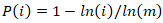
The growing importance of sustainable development and the increase in environmental awareness within society have driven organizations across various economic sectors to pursue more efficient energy management [1].

Despite the global concern with energy efficiency, in the Brazilian context, the evolution of energy management practices has progressed slowly in most municipalities, mainly due to low investments in maintenance and modernization of control systems. However, in the Federal District, the Environmental Sanitation Company of the Federal District (CAESB) has allocated significant resources to modernizing its operational systems and adopting clean energy sources. In the medium term, these initiatives will enable the implementation of real-time automated and optimized control systems, while also helping to reduce operational costs associated with electricity consumption.

In 2022, the Brazilian sanitation sector consumed approximately 12.61 billion kWh of electricity for water supply and 1.72 billion kWh for wastewater services, resulting in expenses of about 9.25 billion Brazilian reais (BRL) [2]. Most of this consumption is attributed to pumping stations. At CAESB, electricity expenses are the second-largest operational cost component. In 2023, the company’s consumption reached around 290.65 million kWh, at a cost exceeding 190 million Brazilian reais (BRL).

Several authors have pointed out, for decades, that energy consumption in most water supply systems could be reduced if appropriate optimization methods were applied [3]. According to these studies, improvements in hydraulic and energy aspects could lead to savings of at least 10% in energy consumption. In recent years, the application of optimization algorithms in water distribution systems has intensified, particularly focusing on methods such as the Genetic Algorithm [4,5,6], Harmony Search [7,8], Particle Swarm Optimization [9,10], Ant Colony Optimization [11], Discrete Dynamically Dimensioned Search (DDDS) [12], and Differential Evolution [13].

Most of these studies adopt reference systems from the literature, which are simpler and have fewer operational units, such as those presented by [14] and [15], either to enable performance comparison between algorithms or due to the unavailability of data required for modeling real systems. Unlike these approaches, the present study applies a real and highly complex Water Supply System (WSS), similar to the one in Vasan [16].

The system under study, called the Descoberto River System, located in the Federal District, is the largest production system in the region in terms of production capacity and population served. Its main operational units include: water intake from the Descoberto River, the Raw Water Pumping Station, the Descoberto Water Treatment Plant (WTP), fifteen ground storage tanks, six elevated reservoirs, seven treated water pumping stations, and nine booster stations. Therefore, it is a highly complex system, both in terms of scale and the number of operational units, which adds further challenges to the optimization process.

Optimization algorithms are generally applied together with hydraulic models, such as EPANET 2.0, to simulate and optimize WSS operations [6,17]. However, traditional hydraulic simulators, such as EPANET 2.0, present high computational processing times, which can make their application to real operations unfeasible, especially in excessively detailed networks. As an alternative, skeletonized or simplified models are used [18], which reduce computational complexity without significantly impairing simulation accuracy.

Due to the complexity of WSS operation optimization, it is also common to apply the Penalty Method, which penalizes infeasible solutions, guides the search toward the feasible solution space, and transforms constrained optimization problems into unconstrained ones by applying penalty coefficients [8,17,19]. Among the strategies adopted by some authors, the so-called “death penalty” stands out, in which solutions that violate constraints receive constant penalties. However, this approach has limitations, as infeasible individuals in the initial population, which would otherwise be discarded, may be essential for obtaining optimized solutions [17].

In this context, Fuzzy logic–based penalties [15] emerge as a promising alternative [20], as they enable different degrees of penalization for each type of constraint violation, providing greater flexibility and efficiency of the optimization process.

Thus, this study aims to primarily develop an optimization model that defines operational rules and minimizes electricity costs in water pumping, using Fuzzy penalties and computational processing time reduction techniques, based on the case study of the Descoberto River System. This study is particularly relevant in the current Brazilian context, marked by low rainfall rates and critical reservoir levels, which have resulted in increased energy costs and directly impacted the tariffs charged to consumers.

2. Methodology

2.1. Characterization of the Descoberto Water Production System

According to CAESB [21], the Water Production System for Urban Supply of the Federal District (SPA) comprises the Descoberto, Corumbá, Torto/Santa Maria/Bananal, Paranoá Lake, Sobradinho/Planaltina, Jardim Botânico/São Sebastião, Brazlândia, Água Quente, Engenho das Lages, Incra 8, Papuda, and Vale do Amanhecer systems. Inaugurated in 2022, the Corumbá system expanded the service areas and increased the company’s potable water production capacity by approximately 15%. Some of these water supply systems are shown in Figure 1.

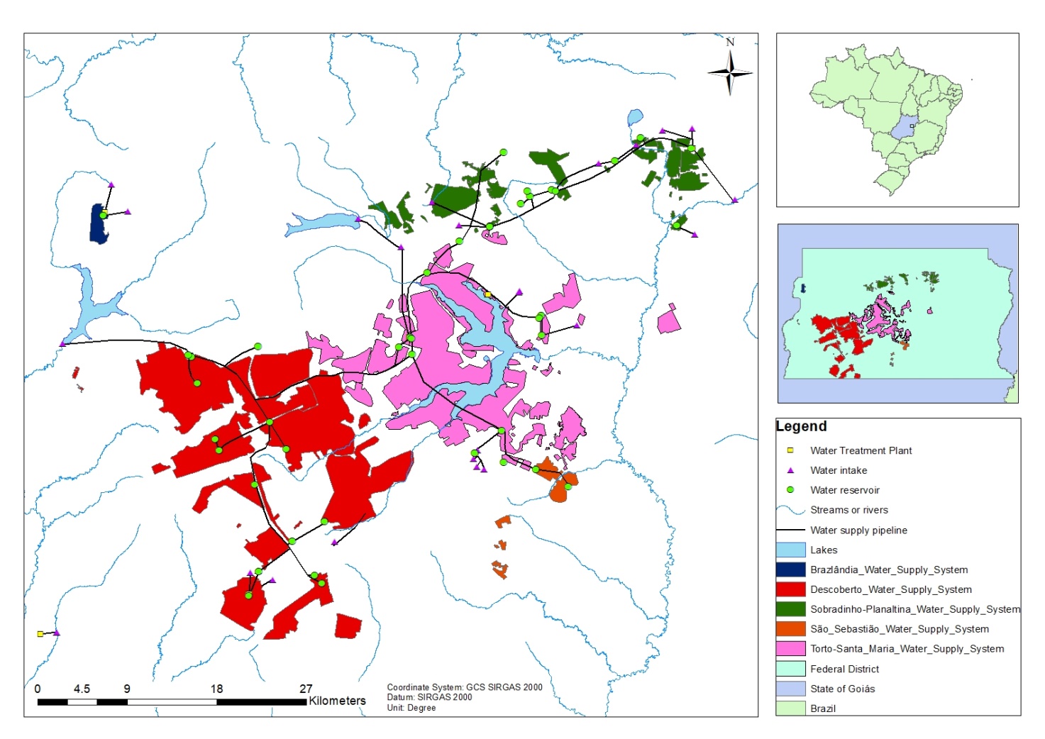
Figure 1. Federal District Water Production Systems

Currently, the Descoberto system is the largest water producer in the Federal District in terms of volume supplied and population served. This system supplies the administrative regions of Ceilândia, Taguatinga, Vicente Pires, Águas Claras, Samambaia, Riacho Fundo I and II, Recanto das Emas, Gama, Santa Maria, Núcleo Bandeirante, Park Way, Candangolândia, Sol Nascente, Pôr do Sol, and Arniqueiras.

The Descoberto water system began operating in 1979, following the completion of the storage dam and raw water pumping station. It was originally designed for a flow rate of approximately 6,000 L/s at the end of its expansion plan [22]. According to the Water, Energy and Basic Sanitation Regulatory Agency of the Federal District (ADASA) [23], in 2024, the system produced an average flow of 3,744 L/s and a maximum flow of 4,223 L/s, which is responsible for 52% of the total water production and for supplying around 60% of the Federal District population.

Water production in the Descoberto system was reduced in 2017 due to changes in the SPA, motivated by the water crisis that affected the region. Since its conception, it is estimated that the system has reached an instantaneous maximum flow of 5,300 L/s on peak consumption days, a value close to its designed maximum production capacity. Operating near design capacity may indicate limitations for implementing optimization strategies, as the higher the level of equipment utilization, the lower the operational flexibility for adopting new operating rules [22].

The main units of the Descoberto system, whose infrastructure includes the Descoberto River intake, the Descoberto River Raw Water Pumping Station, the Descoberto Water Treatment Plant (WTP), fifteen ground reservoirs, six elevated reservoirs, seven treated water pumping stations, and nine booster stations.

Water abstraction for supply is carried out in the Descoberto River, on the border between the Federal District and the municipality of Águas Lindas de Goiás. The Descoberto River Raw Water Pumping Station has five pumping sets, totaling 44,000 hp of installed capacity, of which 27,500 hp are in operation and 16,500 hp are kept in reserve.

The raw water abstracted is pumped by the pumping station to the Descoberto Water Treatment Plant (WTP). After treatment, all treated water is directed to the M Norte 1 Ground Reservoir. From this reservoir, the water is distributed to the other operational units of the system, which are responsible for supplying the different administrative regions. Figure 2 presents a flowchart of the main units of the Descoberto Water Production System.

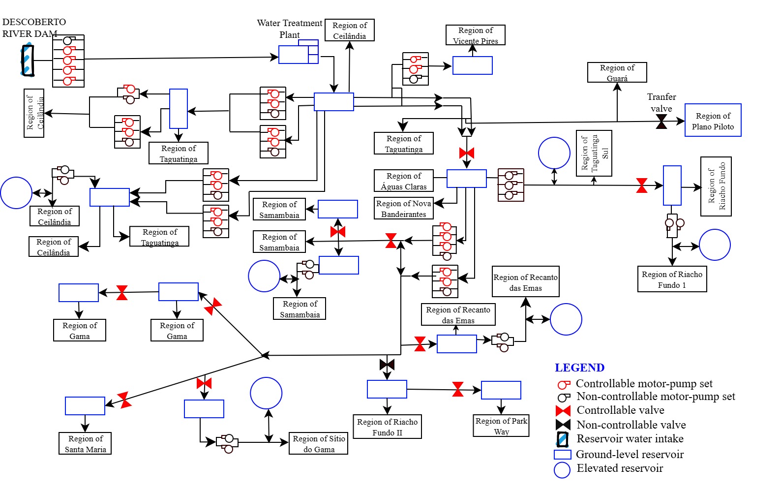
Figure 2. Conveyance flowchart of the Descoberto Water Supply System

In addition to the operational units, the Descoberto System has five main electricity-consuming units, where the ten pumping stations that comprise the optimization problem are located. Each unit has its own electricity supply contract, including characteristics that may or may not be common to other units [22].

2.2. Optimization Model

The optimization model was developed based on a representation of the Descoberto Water Supply System, comprising reservoirs, pumps, and valves, considering a deterministic water consumption regime. The program simulates the operation of a typical day of the system over a 24-hour horizon (from 0:00 to 24:00), aiming to minimize the operational costs of the pumps with hourly resolution. The optimization aims to meet demand without supply failures while respecting operational constraints, such as minimum and maximum reservoir levels, maximum number of pump activations, positive pressure at demand nodes, and the difference between initial and final reservoir levels, all within pre-established limits.

Similarly to Li [6], who proposed optimizing pumping station design to address insufficient pressure issues during peak hours at a railway station and in a municipal committee area, this study adopted a hydraulic modeling–based approach. The authors built a network model, conducted a systematic analysis of the supply system, and applied the NSGA-III algorithm in conjunction with EPANET software to solve a multi-objective optimization problem, simultaneously considering energy consumption and water age in the network, as well as hydraulic constraints such as reservoir levels and node pressures.

In the present study, the methodological basis was the algorithm developed by Gebrim [22], which uses a Simple Genetic Algorithm implemented via the GALib library from the Massachusetts Institute of Technology (MIT), coupled with the EPANET 2.0 hydraulic simulator [24], using the codes available in the Toolkit Library. The adopted methodology also follows the line of research developed by [5,15,25]. The algorithm was implemented in C++ programming language using the Microsoft Visual Studio Express 2012 compiler.

The optimization modeling aims to minimize the electricity costs associated with system pumping, as addressed in studies such as [6,26,27]. The objective function considers the total daily electricity cost, including both the energy consumed by the pumps and the demand cost of the consumer units, in accordance with the blue and green time-of-use tariffs, which differentiate between peak and off-peak periods.

The total electricity cost used in pumping is represented by the objective function (Equation 1), consisting of the sum of the pump consumption costs and the demand cost, the latter divided by 30 to represent the daily value. The demand cost is calculated based on the highest power demanded by each consumer unit during each tariff period of the day (peak and off-peak hours).

(1)

Where: FO(X; Y) = objective function; X = matrix of pumps that are decision variables of the problem; Y = matrix of valves that are decision variables of the problem; Cb = total electricity cost spent on pumping; CC_{(b, t)} = electricity consumption cost of pump b in period t = 1,...,T; u = index of the consumer unit under analysis; U = total number of consumer units (pumping stations) in the problem; CD_(u) = total electricity demand cost of consumer unit u in period t = 1,...,T; b = index representing each pump in the problem; B = total number of pumps in the problem; t = simulation time step under analysis; T = total analysis period.

For the calculation of the objective function presented in Equation 1, the values of electricity consumption were considered at the time intervals during which the pumps remained in operation. These values were classified according to the tariff periods, corresponding to peak hours (higher cost) and off-peak hours (lower cost), as shown in Table 1.

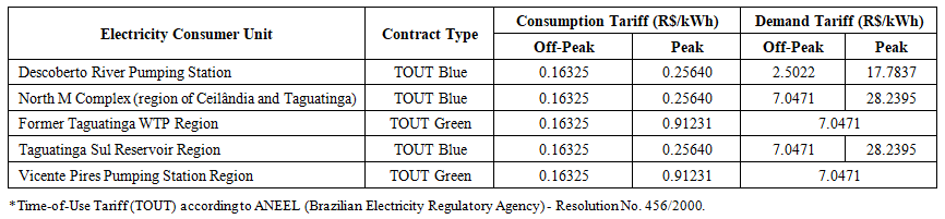
Table 1. Electricity tariff by pumping station analyzed

The optimization problem involves 32 discrete decision variables, corresponding to 22 pumps and 10 valves. Solution encoding was performed using a binary vector representation, in which each component can assume only two states: on (1) or off (0) for pumps; and open (1) or closed (0) for valves. This representation reflects the operational state of each piece of equipment throughout the 24-hour simulation period, according to the approach adopted by [28].

For the present problem, four explicit constraints were considered: (i) positive pressure at demand nodes, with a minimum value of 10 meters of water column (m.w.c.); (ii) water levels in the reservoirs within operational limits, i.e., above the minimum level and below the overflow level; (iii) number of equipment activations below the maximum tolerable limit, which varies according to the size of the equipment; and (iv) difference between the initial and final reservoir levels below an admissible value, to ensure the system’s operational continuity.

A penalty was assigned to each of these constraints, applied to the objective function according to the Penalty Method. The penalties considered were: (P1) reservoir water levels below the minimum limit or above the maximum limit (overflow); (P2) failure to meet demand; (P3) number of pump/valve activations above the tolerable limit; and (P4) difference between initial and final reservoir levels exceeding the admissible value.

Penalty 1 (Equation 2) aims to prevent solutions that result in reservoir levels below the operational minimum, which are necessary to ensure supply continuity. Additionally, this penalty also aims to prevent reservoirs from reaching levels that would cause overflow.

Penalty 2 (Equation 3), in turn, aims to ensure the continuity of water supply by eliminating solutions that would result in shortages. For this purpose, pressures at consumption nodes below 10 meters of water column (m.w.c.), the minimum parameter required to ensure adequate supply, are penalized.

The model presented in [22] employed the Penalty Method, whereby solutions were heavily penalized when certain events occurred. Since the penalization strategy of the fitness function directly and significantly impacts the optimization outcomes, this study proposes a new penalization approach. The implemented strategy gradually penalizes the fitness function through varying levels of violation (degrees of penalization) defined for each constraint, employing fuzzy logic to formulate the penalization equations based on the fuzzification of the variables associated with the constraints. In this framework, the full degree of penalization is represented by a value of 0 or 1, while intermediate values vary according to Equation 6, depending on the analyzed variable and the maximum and minimum limits established for each penalty variable. Further details are provided in Section 2.3.

(2)

Where: P1 = penalty related to the minimum and maximum level limits; j = index of the reservoir under analysis (ranging from 1 to 24); R = total number of reservoirs analyzed (24 reservoirs); T = total analysis period (24 h); t = simulation time step under analysis (ranging from 0 to 23 h); G1_c = full penalty degree applied to P1 (value of 0 or 1); λ₁ = penalty coefficient applied to G1 (value of 10,000); G1_g = gradual penalty degree applied to P1 (depends on the imposed minimum and maximum limits and the level of the reservoir under analysis).

(3)

Where: P2 = penalty associated with the failure to meet demand; t = simulation time step under analysis (ranging from 0 to 23 h); T = total analysis period (24 h); i = index of the consumption node under analysis (ranging from 1 to 35); G = total number of consumption nodes analyzed (35 nodes); D_{(i, t)} = demand at node i at time t (depends on the consumption pattern values of the analyzed node); λ₂ = coefficient applied to Penalty 2 (value of 100); G2_c(i,t) = full penalty degree applied to P2 at each node i at each time t (value of 0 or 1); G2_g(i,t) = gradual penalty degree applied to P2 at each node i at each time t (depends on the maximum and minimum pressure limits from 0 to 10 m.w.c. and the pressure at the node at the analyzed time step).

Penalty 3 (Equation 4) aims to reduce the number of pump and valve activations, which are considered decision variables. Excessive activations compromise equipment durability, affecting proper operation and reducing service life. This penalty consists of two components. The first applies exclusively to pumps and penalizes any shutdown, assigning a value to the penalty corresponding to 1.5 times the pump’s energy consumption in the hour prior to shutdown. Thus, the shutdown has a greater impact on the fitness function than keeping the pump running for an additional hour. In terms of electricity cost, the benefit of turning off a pump for just one hour is lower than the cost associated with the shutdown itself. This indirectly forces the optimization model to avoid solutions in which pumps are switched off and on in short intervals. The second component of the penalty applies to both pumps and valves and aims to eliminate solutions in which equipment is activated more times than a predetermined limit.

(4)

where: P3 = penalty related to the number of pump/valve activations exceeding the tolerable limit; b = index representing each pump in the problem (ranging from 1 to 22); B = total number of pumps in the problem (22 pumps); t = simulation time step under analysis (ranging from 0 to 23 h); T = total analysis period (24 h); CC_{(b, t-1)} = electricity consumption cost of pump b from period t-1 to t (calculated using the data from Table 1); Ac_{(b, t)} = verification of the occurrence of activation of pump b at time t (depends on the maximum and minimum activation limits established in Table 2); G3_c = full penalty degree applied to P3 (value of 0 or 1); λ_3-gn = coefficient applied to Penalty 3 for equipment group n (varies according to Table 2); G3_g = gradual penalty degree applied to P3 (depends on the maximum and minimum limits of activations and the number of activations at the analyzed time step); v = index representing each valve in the problem (ranging from 1 to 10); V = total number of valves in the problem (10 valves); n = group to which the analyzed equipment (pump/valve) belongs (varies according to Table 2).

For the application of this penalty, four equipment groups were defined, classified as follows: pumps of 11,000 hp; pumps of 5,500 hp; pumps with power between 200 and 5,500 hp; pumps with power equal to or less than 200 hp; and valves. For each group, different activation limits and penalty coefficients were established, with the highest coefficient assigned to group 1 and the lowest to group 4, since it is not allowed for higher-power pumps to be activated multiple times per day, according to Table 2.

Table 2. Equipment Groups, Limits, and Penalty Coefficients

Penalty 4 (Equation 5) aims to preserve the initial hydraulic conditions of the system at the end of the daily cycle, ensuring operational feasibility for subsequent simulated periods. This penalty penalizes solutions in which the difference between the initial and final reservoir levels exceeds the maximum limit of 5% of its maximum level. This limit was defined to prevent the problem from becoming excessively restrictive.

(5)

Where: P4 = penalty related to the differences between initial and final levels; j = index of the reservoir under analysis (ranging from 1 to 24); R = total number of reservoirs analyzed (24 reservoirs); T = total analysis period (24 h); t = simulation time step under analysis (ranging from 0 to 23 h); G4_c = full penalty degree applied to P4 (value of 0 or 1); G4_g = gradual penalty degree applied to P4 (depends on the maximum and minimum limits of the differences, ranging from 3 to 5%, between the initial and final levels, and on the level difference at the analyzed time step); λ₄ = penalty coefficient applied to G4 (value of 10,000).

Thus, the fitness function is obtained by adding the penalties to the objective function, which considers the pumping cost combined with the demand-related cost.

The initial level of all reservoirs was set at 98% of the maximum level to provide greater hydraulic benefits and, consequently, increase the operational safety of the storage systems. In addition, the start of operation was established at 06:00 hours. This choice is based on the analysis of [22], which indicated that, at this time, the reservoirs usually reach their maximum levels. Therefore, initialization at this point aims to accelerate convergence to optimal solutions.

2.3. Application of the Fuzzy Approach to Penalties

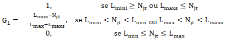
In the model proposed by [22], the penalization strategy used the so-called “death penalty,” which could result in the loss of individuals that would contribute to improving the optimized solution. This approach could lead to the elimination of promising solutions, preventing progress toward optimization. Considering that the way the fitness function is penalized directly and significantly influences the search for optimized solutions, a new penalization strategy was implemented. This new approach is based on the methodology proposed by [7,15,20], using Fuzzy logic for the formulation of penalization equations, by the fuzzification of the variables associated with the constraints.

The concept of Fuzzy logic was applied to all penalties, with penalty degrees ranging from 0 to 1. These degrees were subsequently multiplied by their respective penalty coefficients, allowing for a more gradual and realistic penalization. Trapezoidal membership functions were adopted to define the penalty degrees of all variables related to the constraints.

The choice of this format is justified by its proven suitability in previous studies, such as [29,30], in which the trapezoidal function proved effective for variables such as reservoir levels, pressures at consumption nodes, and the number of pump and valve activations. Figure 3 illustrates the application of the Fuzzy concept to Penalty 1.

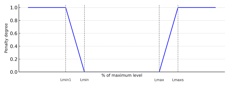
Figure 3. Application of the Fuzzy concept to Penalty 1

Equation 6 represents the penalty degree corresponding to Penalty 1, used in the optimization model.

(6)

Where: G₁ = penalty degree applied to Penalty 1 (dimensionless); L_max = lower maximum level limit (%); L_maxs = upper maximum level limit (%); N_jt = level of reservoir j at time t (%); L_min = upper minimum level limit (%); L_mini = lower minimum level limit (%).

According to normally observed operating conditions, the minimum limit considered for the application of this penalty was set at 10% of the maximum level of each reservoir (L_mini). The maximum limit for the application of the penalty was 98% of the reservoir’s maximum level (L_maxs). This limit was established based on operational records from CAESB. Meanwhile, L_min ranged between 12% and 15%, and L_max ranged between 93% and 96%.

The fuzzification procedure, as well as the derivation of the equations related to the penalty degrees, was likewise applied to Penalties 2, 3, and 4, respectively, ensuring the uniformity of the method applied across all stages of the analysis.

2.4. Hydraulic Model

The hydraulic simulator used for the optimization of the Descoberto Water Supply System (WSS) was EPANET 2.0. The conceptual hydraulic scheme used in the study was based on the dynamic model proposed by [22], with some simplifications. In the literature, several studies on water supply system optimization use a reference system called Anytown, which has a reduced number of operational units, as in the works of [27,31,32]. On the other hand, studies such as [33,34] simulate real and more complex systems.

The scheme of the Descoberto System used in this study includes a total of 273 nodes, consisting of: 23 reservoirs with variable levels, 1 fixed-level reservoir, and 35 consumption nodes. It also comprises 331 hydraulic links, of which 267 are pipelines, 47 are pumps, and 17 are valves. This set represents a high number of operational units, giving the model greater complexity compared to systems commonly adopted in the literature, which is a significant differentiating factor of this study. The hydraulic model of the Descoberto WSS is illustrated in Figure 1.

The original hydraulic model had a high number of nodes and links, which significantly increased the processing time during optimization. Therefore, a simplification or skeletonization process was adopted, as applied in previous studies such as [18,35,36], to reduce computational time without compromising the hydraulic representativeness of the system. This simplification was performed through the creation of equivalent links by combining series and parallel links. For this purpose, the equivalent length equations presented by [37] were used. It is important to emphasize that no operational unit, nor any consumption node, was simplified during the process, ensuring that critical elements for system operation and control were preserved.

The EPANET 2.0 model used monthly average consumption values, which implies that the operational rules adopted represent an average system operating condition. The model calibration was performed through a 24-hour extended simulation, using a known operational rule previously applied in the real system. The calibration process was conducted iteratively, with adjustments to head loss parameters, pump curves, and consumption patterns until the simulated reservoir levels approximated the observed field values. Model validation was not performed, as this structure was previously adopted by the company and considered already validated for operational purposes.

2.5. Optimization Algorithms

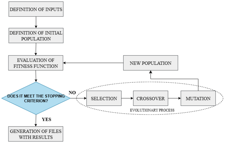
Different algorithms were tested to optimize the operational electricity costs of pumping in the Descoberto Water Supply System (WSS). The algorithms evaluated were the Genetic Algorithm (GA), Dynamically Dimensioned Search (DDS), and Differential Evolution (DE). The GA, originally proposed by Holland [38], was selected for the main simulation, as it and its extensions, such as NSGA-II (Non-dominated Sorting Genetic Algorithm), are widely used in the literature for WSS optimization problems [6,15,27,39,40].

Among evolutionary algorithms, the Genetic Algorithm (GA) was one of the first to be applied to the optimization of water supply systems (WSS). GAs are computational search and optimization methods for complex problems, inspired by the mechanisms of natural selection and survival of the fittest, as described in Charles Darwin’s Theory of Evolution (1859).

The basic operational cycle of the simple genetic algorithm (Figure 4) begins with the creation of the initial population, which consists of a set of solution vectors representing the initial values of the decision variables. This population can be generated randomly or defined by the user. The fitness function is then evaluated for each vector. Subsequently, it is verified whether the stopping criterion has been met; in this case, the criterion is the number of GA generations. If the criterion is satisfied, the algorithm terminates; otherwise, the processes of selection, crossover (recombination), and mutation are applied to generate a new population for the next evaluation of the fitness function. This cycle continues until the stopping criterion is met.

Figure 4. Basic Operation of the Genetic Algorithm (GA)

The GA process begins with the definition of the inputs (Step 1), which includes all general data required for the optimization. Two routines were employed for this purpose: the first opens the EPANET 2.0 input file to account for the number of nodes, pipes, and reservoirs, while the second reads a text file containing information such as the genetic algorithm parameters (selection type, crossover type, crossover probability, mutation type, mutation probability, population size, number of generations, and random seed), the penalty coefficients, the number and identification of problem variables (pumps and valves), the simulation time (number of hours), and the initial reservoir levels.

In Step 2, the initial population (a set of solution vectors) is generated randomly, with the same initial solution applied across all simulations to ensure a consistent starting point for comparison, since the initial solution is a critical factor affecting the optimization outcomes.

Step 3 involves the evaluation of the fitness function. During the first evaluation, the function is calculated using the initial solution vector. In subsequent evaluations, the GA-generated solution vectors, along with the initial reservoir levels, are input into the EPANET2.0 hydraulic simulator. The simulator performs the hydraulic computations, producing variables such as pressure, flow, energy consumption, equipment states, and demand, which are then used by the optimization model to calculate the fitness function. This execution method, which leverages EPANET2.0’s programming toolkit, allows access to partial data throughout the dynamic simulation and is commonly employed in optimization studies.

In Step 4, the stopping criterion is evaluated, which in this study corresponds to the number of GA generations. If the criterion is met, the algorithm selects the best solution found and generates detailed output files containing energy consumption, reservoir levels, equipment activations, constraint violations, and associated costs. If the stopping criterion is not met, the current population undergoes the GA evolutionary process (Step 5), consisting of selection, crossover, and mutation, to generate a new population for the next fitness function evaluation.

The DDS, developed by Tolson and Shoemaker [41], was adopted due to its simplicity compared to other evolutionary and metaheuristic algorithms, as discussed by [42]. It is a non-population-based algorithm designed to efficiently find good solutions. DDS is not sensitive to the scale of the objective function, has only one parameter — the scalar neighborhood size perturbation parameter (r) — and is applicable to discrete, continuous, and mixed variables. Due to these characteristics, it is particularly recommended for problems where objective function evaluation requires significant computational processing time.

The DDS is a stochastic single-solution algorithm based on global heuristic search, designed to identify high-quality global solutions within a maximum limit of objective function evaluations, which serves as the algorithm’s stopping criterion. In essence, the algorithm performs a global search during the early stages of optimization and progressively shifts toward a more local search as the number of iterations approaches the maximum allowed evaluations.

The operational steps of the DDS algorithm are illustrated in Figure 5. According to [41], the first step involves defining the algorithm inputs, which include the penalty coefficients; the number and identification of problem variables (pumps and valves); the simulation time (number of hours); the initial reservoir levels; the parameter that determines the perturbation neighborhood size (r); the maximum number of objective function evaluations (m); the vectors of upper and lower bounds of the decision variables (xmax and xmin, respectively); and the vector of initial solutions, x₀ = [x₁, x₂, …, xD], representing the initial values of each decision variable.

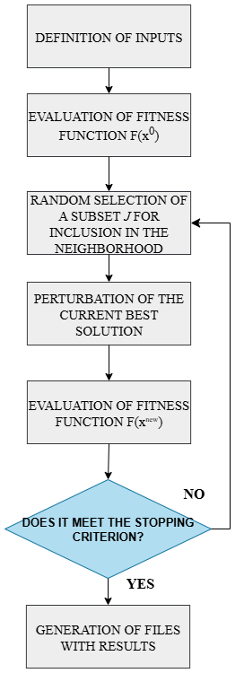
Figure 5. Basic Operation of the DDS

In the second step of the DDS algorithm, the fitness function is evaluated using the initial solution vector (x₀), yielding F(x₀) at iteration i. Since this is the first evaluation, F_best is assigned to this solution and x_best to the vector x₀. The fitness calculation requires performing the hydraulic simulation using EPANET2.0 via its function library (toolkit), with the initial solution vector representing a 24-hour operational rule.

The hydraulic simulation execution follows the same logic as in the GA. In Step 3, a random subset J of the D decision variables is selected for inclusion in the neighborhood {N}. Initially, the probability of including each decision variable in {N} is computed as a function of the current iteration, as shown in Equation 7. Then, for d = 1, 2, …, D, variable d is added to {N} with probability P. If {N} is empty, a random variable d is selected and added to {N}.

(7)

Where: P = probability of including each variable in {N}; i = iteration; m = maximum number of objective function evaluations.

In the next step, the current best solution vector (x_best) is perturbed for all j = 1, 2, …, J decision variables in {N}. This perturbation of the current best solution generates a candidate solution vector (x_new).

In Step 5, the fitness function F(x_new) is evaluated using the candidate solution vector (x_new), and the current best solution is updated. If F(x_new) ≤ F_best, then F_best = F(x_new) and x_best = x_new.

In Step 6, the stopping criterion is checked. If the criterion is satisfied, the algorithm outputs the results to files; otherwise, the algorithm returns to Step 3.

The Differential Evolution (DE) algorithm, proposed by Storn and Price [43], was also considered due to its fast convergence to optimal solutions, as demonstrated in previous studies [42,44,45,46].

According to Storn and Price [43], optimization performed by DE is quite similar to that of the GA, with mutation, crossover, and selection operators. The names of the operators are similar to those used in GAs; however, there are significant differences in the order of application and in their implementation, particularly in the mutation process, which involves creating a mutant solution through the selection of three random solutions (x_r0, x_r1, and x_r2) from the current generation.

The DE algorithm begins with the selection of a random solution to be replaced (target vector), along with another solution called the principal vector, x_r0,g (base vector). Then, two additional solutions (x_r1,g and x_r2,g) are randomly selected, and the difference between x_r1,g and x_r2,g is calculated and scaled by a factor F. The mutation of x_r0,g consists of adding the scaled difference vector to the base vector, resulting in a mutant vector (Equation 8). This type of mutation represents the classical mutation strategy of DE.

(8)

Where: x_r0,g = base (principal) solution; x_r1,g and x_r2,g = randomly selected solutions; v_0,g = generated mutant solution; F = mutation factor.

The crossover operation between the target vector and the mutant vector involves replacing the parameters of the target vector with those of the mutant vector, with each parameter having a probability CR (crossover probability) of being replaced. The result of this operation is the trial vector u_0,g.

Following the crossover, a selection process is carried out between the target vector and the trial vector, based on the fitness function. In addition to the population size and the maximum number of generations, the DE algorithm requires the definition of two additional parameters: the mutation constant F and the crossover constant CR, both ranging from 0 to 1.

Similar to DDS, the DE optimization model incorporates multiple functions, including a main function. Besides invoking other functions such as the DE core function, the fitness evaluation function, and auxiliary routines, the main function also defines the input data. These inputs include the penalty coefficients, simulation time in hours, initial reservoir levels, population size, number of generations, mutation strategy, the number and identification of decision variables (768 variables) along with their upper and lower bounds, as well as the mutation F and crossover CR constants. This constitutes the first step in the algorithm’s operation. In Step 2, the initial solution vector is defined, assigning values to all decision variables. These values are then used to evaluate the fitness function (Step 3).

In the subsequent step, the algorithm checks whether the evaluation criterion has been met, which in this case corresponds to the number of generations. If the criterion is not satisfied, the processes of mutation, crossover, and selection are performed to generate a new population (set of solutions) and re-evaluate the fitness function. Once the evaluation criterion is satisfied, the algorithm simulates the best solution, generates detailed output files with the results, and terminates the process.

The performance of the tested algorithms was analyzed using the following performance indicators: cost (objective function), fitness, and computational time.

The parameters of each algorithm were mostly defined based on sensitivity analyses, as suggested by Dandy [47], except for the GA parameters, which followed the values defined and calibrated by Gebrim [22], as it involves the same optimization problem. For all algorithms, an initial population size of 10 was adopted, which is a value that produced the best results in Gebrim’s previous simulations [22], and a total of 1,000 generations, totaling 10,000 objective function evaluations.

The penalty coefficients used were also based on the values employed by Gebrim [22], considering the sensitivity analysis already performed and the similarity of the studied problem. The following coefficients were adopted: λ1 = 10,000; λ2 = 100; λ3_g1 = 10,000; λ3_g2 = 10,000; λ3_g3 = 2,000; λ3_g4 = 1,000; λ4 = 10,000. For the GA, the genetic operators previously calibrated by Gebrim [22] were used: tournament selection, single-point crossover, simple mutation, crossover probability of 0.7, and mutation probability of 0.004.

According to Tolson [12], the only parameter of DDS is the perturbation neighborhood size (r), with a default value of 0.2. Given the complexity of the optimization problem and the sensitivity of results to the adopted parameters, a sensitivity analysis of parameter r was conducted, varying between 0.1 and 1. For the DE algorithm, different combinations of parameters F and CR were tested through sensitivity analysis. The values tested ranged from 0.5 to 1, using the classical DE/rand/1/bin strategy, widely referenced in the literature. Additionally, the seeding technique was employed in population initialization to accelerate convergence to good solutions, especially considering the high processing time required by the problem. The initial solution was obtained through a simulation with 100,000 evaluations, based on a real operational rule used by the company in the Descoberto water supply system.

2.6. Input and Output Data of the Optimization Model

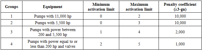
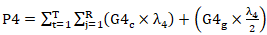
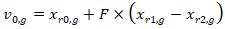
The input data considered for the simulation of the optimization model were as follows:

• Algorithm parameters: For the GA, the genetic operators previously calibrated by Gebrim [22] were used, as described in the previous section. For the DDS, a sensitivity analysis of the parameter was performed, setting the value of r = 0.3. For the DE algorithm, different combinations of the parameters F and CR were tested through sensitivity analysis, with the best results obtained for F = 0.6 and CR = 0.8.

• Penalty coefficients: Defined based on the values used by Gebrim [22], considering the sensitivity analysis already conducted and the similarity to the problem under study, with the values presented in the previous section.

• Initial solution (rule): Based on an actual operational rule used by the company responsible for the Rio Descoberto water supply system, aimed at accelerating the model processing. The initial fitness of this rule corresponds to 1,980,000. The rule consists of a set of 768 binary variables (0 or 1), where 0 represents the off/closed state and 1 the on/open state.

• Number of objective function evaluations: A population size of 10 was considered — a value that produced the best results in Gebrim's simulations [22] — and 1,000 generations, totaling 10,000 objective function evaluations.

• Maximum and minimum limits for applying the degrees of penalization in the fuzzy approach, according to the values previously presented.

• Data for calculating electricity costs, as shown in Table 2.

In total, the system under study consists of 5 energy-consuming units, where 10 pumping stations are installed, totaling 22 pumps involved in the optimization problem. The calculation was performed considering the location of each pumping station and its respective consumer unit, according to Equation 1, which presents the objective function.

Additionally, input data were required in the EPANET 2.0 software, including:

• Hourly consumption data over 24 hours, defined based on monitoring records from the water supply company and data from Gebrim [22], considering it is the same water supply system.

• Start of operation: set at 06:00, as Gebrim [22] verified that at this time the reservoirs reached their maximum level, and it corresponds to the actual start of operation, which approximately coincides with the arrival of the operators at the company.

• Initial reservoir levels: set at 98% of the maximum level, aimed at providing better hydraulic benefits and, consequently, greater operational safety.

Based on the input data and the simulations performed, the model was able to generate the following output data:

• Energy consumed in pumping operations.

• Electricity costs.

• Node pressures.

• Reservoir levels.

• Water flows in the network segments.

• Algorithm processing time.

• EPANET processing time.

• Total processing time.

• Objective function value and fitness function value.

• Penalty values.

• Operating status of pumps (on/off) and valves (open/closed), with on/open represented by 1 and off/closed represented by 0, as shown in Figure 6. This set is also referred to as the operational rule.

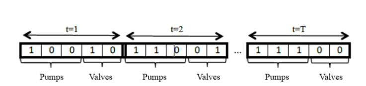
Figure 6. Example of the operational rule representation for three pumps, two valves, and optimization period T. Source: [22]

3. Results and Discussion

The optimization model of the Water Supply System (WSS) was developed to minimize the total electricity cost for the operation of the Descoberto System over a 24-hour period. The model formulation considered the calculation of the energy consumption of each pump, the demand-related cost, and penalties associated with operational variables such as pressures at consumption nodes, reservoir levels, and the number of pump and valve activations. For each solution generated by the algorithm, which is represented by an operational rule, the model performs a hydraulic simulation using the EPANET software. This provides the values of the hydraulic variables, which are then used by the algorithm to calculate costs and penalties. Based on these results, the fitness function is evaluated, and a new rule is generated, repeating the process until all predefined function evaluations are executed.

The model operation is based on penalizing rules that are operationally unfeasible. This includes activations that would result in pressures outside the limits established by technical standards, reservoir levels that are too high or too low, excessive pump starts, as well as variations between minimum and maximum levels exceeding a predetermined limit. Thus, the model ensures that optimized solutions respect the operational constraints of the real system.

Simulations showed that, although the model was capable of finding solutions with reduced operational costs, many of these solutions would not be practically feasible. This occurs because some operational rules generated, while economically efficient, did not meet safety and operational reliability criteria. Such rules were automatically discarded by the optimization process. At the end of the simulations, the model was able to identify the operational rule closest to the ideal, reconciling practical feasibility with the lowest possible energy cost within the established operational limits. These results demonstrate the potential of the model as a decision support tool for the efficient operation of water supply systems.

3.1. Optimization Model

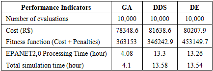
To obtain the operational rules through the optimization algorithms, a fixed number of 10,000 fitness function evaluations was defined, with all algorithms starting the simulation from the same initial solution.

The results obtained from the simulations carried out using the GA, DDS, and DE optimization algorithms, considering the same number of objective function evaluations (10,000), are presented in Table 3.

Table 3. Comparison of the performance of the optimization algorithms

The lowest cost obtained was R$ 78,348.6, in the optimization performed using the GA. The operational cost of the water supply system depends both on the demand of the consumer units and on the energy consumption of the pumps, which is calculated as the product of energy consumption and the applied tariff, varying between peak and off-peak periods. Thus, the lower value of the objective function can be explained by the fact that the solution found involves a smaller number of pumps in operation during these tariff periods.

From Table 3, it can be observed that the processing time of the hydraulic simulation (EPANET2.0 time) constitutes a critical factor for the speed of the optimization process, as it accounts for a large portion of the total execution time.

It was also noted that the processing time required to obtain the optimized rule using DDS and DE is at least three times higher than that obtained with the GA. This difference can be attributed to the programming languages used, since the first two were implemented in MATLAB, an interpreted language that requires longer execution time, whereas the latter was implemented in C++, a compiled language and therefore more efficient in terms of processing.

The Genetic Algorithm (GA) showed the fastest convergence speed in the initial iterations compared to the DDS (Dynamically Dimensioned Search) and DE (Differential Evolution) algorithms. However, the GA did not converge to the best fitness within the limit of 10,000 evaluations. The DE showed similar performance to the GA in the early iterations but displayed poorer convergence in the final evaluations, possibly due to its predominantly global nature, a characteristic also applicable to the GA.

On the other hand, the DDS, although it converged more slowly, was the only algorithm to reach the best fitness. This can be attributed to its search strategy: initially global and progressively more local as the number of evaluations approaches the maximum set. All algorithms proved to be suitable for optimizing the Descoberto System. However, the DDS stood out for presenting more consistent results in terms of fitness and for its ease of use, as it depends on only one parameter. Despite this, the GA was selected for subsequent simulations because it produced the lowest pumping cost.

Simulations indicated that the application of the Fuzzy approach to penalties played a relevant role in improving the model’s performance. This approach enabled the gradual exclusion of infeasible solutions, instead of discarding them outright. Consequently, the model avoided premature trapping in local minima, leading to a more effective evolution of the fitness function. In addition, the Fuzzy penalization resulted in lower electricity costs compared to rigid penalties (“death penalty”), which completely eliminated rules with high penalties, even when they had the potential to improve the objective function.

Considering that hydraulic models with multiple pumps, valves, and reservoirs require long processing times, skeletonization and seeding strategies were adopted. The skeletonization of the hydraulic model — through segment simplification — contributed to a 20.2% reduction in total processing time (equivalent to 50 minutes) compared to the complete model. This gain is particularly relevant, as most of the processing time is consumed by hydraulic simulations, not by the execution of the optimization algorithm itself. The time was not reduced further due to the high complexity of the Descoberto system, which has many operational units that cannot be simplified, in addition to the model already being pre-simplified.

The seeding technique also contributed positively, allowing the algorithm to start the optimization from a real operational rule — already hydraulically feasible — with pressures, levels, and activations compatible with practical operation. As a result, computational effort was concentrated on searching for lower energy costs. This approach was able to generate solutions with better fitness in less time, as also observed in the work of Savić [39], which demonstrated that using real rules as a starting point outperforms the performance obtained with random solutions, both in quality and computational time.

3.2. Operational Rules

The optimized rule was obtained from the application of the Genetic Algorithm (GA), associated with Fuzzy penalization, using the simplified hydraulic model and the seeding technique for initialization. This combination allowed accelerating the model’s convergence and ensuring greater operational feasibility of the solutions. The final rule found did not result in pressures below 10 m.c.a. nor in reservoir levels outside the predefined limits, thus ensuring the continuity of supply over the 24-hour simulation and the applicability of the solution to the real system. However, a total of 26 activations above the recommended limit was observed, which is considered high for the practical operation of Water Supply Systems (WSSs).

The pumping cost for the reference rule practiced by the company at the time of the simulation was R$ 85,934.50, while the cost associated with the optimized rule was R$ 81,327.50 — representing a savings of 5.3%. Although significant, this reduction could have been even higher if not for the already high efficiency present in the Descoberto System. It is noteworthy that the company has a technical team dedicated to managing energy consumption and that the Descoberto system alone operates near its structural limit.

The total operating cost of the WSS comprises the demand cost of the consumer units and the consumption cost of the pumps, which depends directly on the operating time and the energy tariff, varying between peak and off-peak periods. The savings observed in the optimized rule are related to the strategy adopted by the model, which prioritized a smaller number of pumps in operation, both during peak and off-peak periods. Consequently, the number of activations increased, aiming to maintain other criteria within the stipulated penalty limits.

The highest-power pumps, located at the Raw Water Pumping Station (5,500 and 11,000 hp), were responsible for a significant portion of the costs: 0.79% in the optimized rule, 0.83% in the reference rule, and 0.81% in the rule presented by Gebrim [22]. These values confirm that high-power pumps have a great impact on energy costs and, therefore, must be operated with special attention to minimize pumping costs, given their critical role in conveying water throughout the system. In contrast, lower-power pumps (100 and 150 hp) had an insignificant impact on the total cost, even when operating for prolonged periods: 0.011% (optimized rule), 0.006% (reference), and 0.009% [22]. This demonstrates that their continuous operation does not represent a significant increase in costs, allowing greater operational flexibility without impairing economic efficiency.

Figures 7 and 8 illustrate the comparison among three operational strategies: the optimized rule proposed in this study, the reference rule adopted by the company at the time of the simulation, and the rule obtained by Gebrim [22]. Figure 7 shows the four pumps of the raw water pumping station, with powers between 5,500 and 11,000 hp, while Figure 8 displays smaller pumps (100 to 150 hp). Pumps in operation are represented in blue. In the reference rule, there is a tendency for continuous operation or few maneuvers, as in the case of pumps B2_AB, B1_AB, and B4_AB (Figure 7). This strategy aims to reduce mechanical wear of the equipment, prioritizing a lower number of activations. In all analyzed rules, there is a clear tendency to avoid peak hours (6 p.m. to 8 p.m.), which have the highest energy tariffs, as a way to reduce operational costs. Although the optimized rule resulted in a higher number of activations, all high-power pumps remained within acceptable operating limits.

Figure 7 shows a greater tendency to avoid pump activation during peak hours in the reference rule. In the optimized solution, whose objective is the minimization of operational costs (objective function), the same strategy is also adopted.

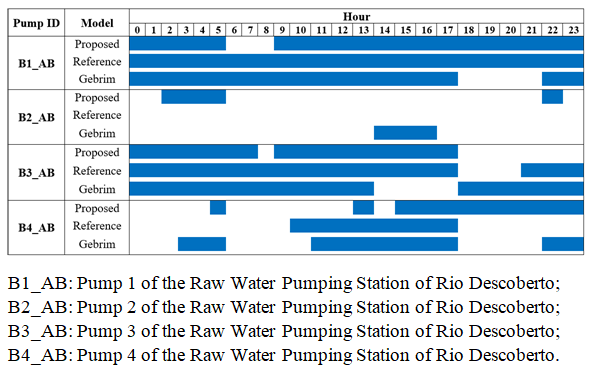
Figure 7. Operational rules for pumps with power equal to 5,500 and 11,000 hp

However, it can be noted that, in some cases, both the optimized rule and Gebrim’s rule [22] have pumps activated during this time interval. This is due to conflicts between the cost-minimization criterion and the penalties associated with reservoir levels. In certain situations, pump activation during peak hours becomes necessary to maintain levels within acceptable operational limits (penalty 1) and to ensure that the initial and final reservoir levels are similar at the end of the simulated period (penalty 4).

An excessive number of activations was observed for the lower-power pumps and the valves, exceeding the recommended operational limit (Figure 8), both under the application of the optimized rule and the rule proposed by Gebrim [22].

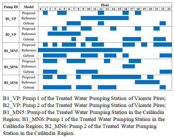
Figure 8. Operational rules for pumps with power equal to 100 and 150 hp

This high frequency of activations can be attributed to the lower weights assigned to the penalties for these classes compared to higher-power equipment. In particular, situations were identified where some pumps operate for only one hour before being turned off, which is a pattern that is unusual and technically inadvisable for water supply systems (WSSs) due to the risk of premature equipment wear.

A notable case occurred with Pump 1 of the Vicente Pires Treated Water Pumping Station, whose total daily operating time was extremely low. Even in scenarios where energy costs or associated penalties were reduced, the high number of activations may not justify the operational damages caused. Modifying the penalty coefficients proved effective in reducing activations, but only to a limited extent. Additionally, these changes resulted in an increase in penalties more critical to operation, such as those related to reservoir levels outside established limits.

Despite these limitations, it is important to highlight that the maneuvers simulated by the model can be technically feasible within the system context, considering that many pumps operate with automatic activations controlled by CAESB. However, the operational feasibility of changing the operating rules for the Descoberto System may be affected due to the high number of activations required, which tends to accelerate wear on pumps and valves in the medium and long term.

The main contribution of the optimization model lies in its ability to quickly identify new viable operational rules, considering the complexity and scale of the system. This capability becomes especially relevant in view of planned maintenance and modifications for the Rio Descoberto System, including its interconnection with the Corumbá IV System.

In its current form, the model allows validation of rules previously established by operators and prediction of the system’s operational behavior in response to these new rules, including the estimation of associated pumping costs. With additional improvements, such as limiting the number of activations and incorporating a demand forecaster, the model could be used in the future to define real-time operational rules.

3.3. Reservoir Water Levels

The reference rule resulted, at the end of the simulated period, in water levels lower than those at the start of the simulation in some cases, as observed in the Riacho Fundo reservoir (Figure 9). According to Gebrim [22], this behavior may indicate that, in real operations, system control is not based solely on the condition that the final reservoir level must be greater than or equal to the initial level. Instead, it is assumed that the initial level is sufficient to support the daily consumption cycle. This principle is also observed in the rule proposed by Gebrim [22], in which reservoir operation starts at 30% of the maximum level and ends at 79%. This demonstrates that the operation aims to ensure that daily demand is met safely, even if the levels do not return exactly to the initial condition by the end of the day.

These results point to the need to consider more flexible operational strategies in optimization models, better reflecting real system practices, especially in contexts where the initial and final reservoir volumes do not need to match, as long as daily supply is ensured.

At the end of the simulated period, the reference rule resultedin water levels lower than those at the start of the simulation in some cases, as observed in the Riacho Fundo reservoir (Figure 9). According to Gebrim [22], this behavior may indicate that, in real operation, system control is not based solely on the condition that the final reservoir level must be greater than or equal to the initial level. Instead, it is considered that the initial level is sufficient to support the daily consumption cycle. This principle is also observed in the rule proposed by Gebrim [22], in which the reservoir operation starts at 30% of the maximum level and ends at 79%. This demonstrates that the operation aims to ensure daily demand is met safely, even if levels do not return exactly to the initial condition by the end of the day.

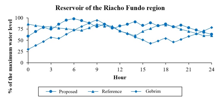
Figure 9. Water Levels in the Riacho Fundo Reservoir

These results highlight the need to consider more flexible operational strategies in optimization models, better reflecting real system practices, especially in contexts where the initial and final reservoir volumes do not need to match, as long as daily supply is ensured.

As shown in Figure 10, for the M Norte 2 reservoir, the optimized rule provides higher water levels in the reservoirs compared to the reference rule and Gebrim’s rule [22]. Thus, the storage capacity is better utilized, helping to prevent depletion or approaching critical operating levels. Maintaining high reservoir levels under the reference rule reflects the operators’ concern for the system’s operational safety. In the optimized rule, the high levels recorded in most reservoirs are also related to the initial simulation condition, which started from an almost full state, imposed by penalties associated with low levels.

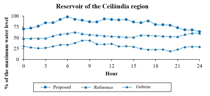
Figure 10. Water Levels in the Ceilândia Reservoir

The water levels obtained under the optimized rule are operationally viable and, in many cases, higher than those of the reference rule throughout the 24-hour simulated operation. This behavior can be considered an advantage of the optimization model, as higher reservoir levels increase operational safety and system resilience, ensuring supply even in emergency situations. However, it was observed that this increase in levels is directly associated with a higher number of pump activations. In other words, to maintain the higher levels forecasted by the optimized rule, the model required more frequent operation of the pumping units throughout the day.

The computational processing time for the simulation was 1.09 hours, considered low, especially given the complexity of the analyzed system. This performance can be attributed to the fact that the simulation started from a known and operationally acceptable solution—already considered a good initial configuration—rather than from a random solution. This approach contributed to reducing the number of iterations needed during the optimization process.

The simulations also revealed that EPANET 2.0 accounts for most of the code’s processing time. It was observed that when real operational rules—tending to be close to hydraulic equilibrium—are used, the number of iterations required to solve the hydraulic balance equations decreases. Consequently, the total simulation time is reduced. This underscores that processing time is directly related to the quality of the solutions generated in each evaluation during optimization.

4. Conclusions

This study developed an optimization model for the pumping operation of the Rio Descoberto Water Supply System, located in the Federal District, using Genetic Algorithms (GA) in conjunction with the EPANET 2.0 hydraulic simulator and Fuzzy Logic. The results demonstrated that system optimization allows for a reduction in electricity costs while respecting established operational constraints. Moreover, the model proved capable of rapidly establishing operational rules close to the optimum, which is promising in scenarios involving system modifications, including the potential integration of the Corumbá IV Water Production System into the Rio Descoberto System—a possibility to be explored in future studies.

The application of the optimized operational rule resulted in a 5.3% reduction in energy costs compared to the simulation of the reference rule. Additionally, higher reservoir levels were achieved, contributing to increased operational safety, further reinforcing the model’s potential for practical application. However, the high number of pump and valve activations observed in the simulations represents a significant limitation, as such behavior is undesirable in real operations due to the risk of equipment wear.

Although the proposed model does not use a multi-objective approach, the results indicate that its application in real operations is feasible, particularly as it produces solutions close to the operational conditions currently adopted. This is reflected in aspects such as the maintenance of reservoir levels, adequate supply pressures, and relatively low processing time (1.09 hours), considering the system’s complexity and the number of evaluations performed.

For real-time implementation, however, additional techniques would need to be incorporated, such as mechanisms to reduce the number of activations and the development of a demand forecaster—here considered as previously known, but in practical operations, subject to variations. Furthermore, complementary studies are recommended, including hydraulic reliability analyses of the system and the formulation of specific rules for operational emergency situations, to enhance the robustness and applicability of the proposed model.

ACKNOWLEDGEMENTS

The authors acknowledge the Coordination for the Improvement of Higher Education Personnel (CAPES) for granting the scholarship to the first author and the Environmental Sanitation Company of the Federal District (CAESB) for providing the data used in this research.

References

[1]  Bluszcz, A and Manowska, A., 2020, Differentiation of the Level of Sustainable Development of Energy Markets in the European Union Countries, Energies, 13(18), 1-20.
[2]  SNIS (2023). Diagnóstico Temático Serviços de Água e Esgoto: Visão Geral ano de referência 2022. [Online]. Available: https://www.gov.br/cidades/pt-br/acesso-a-informacao/acoes-e-programas/saneamento/snis/produtos-do-snis/diagnosticos/DIAGNOSTICO_TEMATICO_VISAO_GERAL_AE_SNIS_2023.pdf.
[3]  James, K., Campbell, S. L., and Godlove, C. E., Água e Energia: Aproveitando as Oportunidades de Eficientização de Água e Energia Não Exploradas nos Sistemas Municipais, 1st ed. Washington, DC: Alliance, 2002, 160 p.
[4]  Qin, X., Luo, Y., Chen, S., Chen, Y., and Han, Y., 2022, Investigation of Energy-Saving Strategy for Parallel Variable Frequency Pump System Based on Improved Differential Evolution Algorithm., Energies, 15 (15), 5360 – 5373.
[5]  Ramani, K., and Umamahesh, N. V., 2024, Multi-criteria decision-making methods for optimal design of intermittent water distribution network., Water Supply, 24 (4), 1176 – 1195.
[6]  Li, R., Wang, H., Xin, K., and Tao, T., 2024, Multi-objective optimization design of integrated pump station based on NSGA-III., Water Supply, 24 (8), 2866 – 2881.
[7]  Geem, Z.W., 2015, Multiobjective optimization of water distribution networks using Fuzzy theory and harmony search, Water, 7(7), 3613–3625.
[8]  De Paola, F., Pugliese, F., Fontana, N., Giugni, M, 2025, A new Digital Harmony Search algorithm for optimizing Pump Scheduling in Water Distribution Networks., Water Research X, 27, 1-11.
[9]  Torkomany, M., Hassan, H. S., Shoukry, A., Abdelrazek, A. M., and Elkholy, M., 2021, An Enhanced Multi-Objective Particle Swarm Optimization in Water Distribution Systems Design., Water, 13 (10), 1334 – 1345.
[10]  Wang, D., Liu, Z., Zhang, D., and Liu, X., 2024, Prediction of water consumption in Beijing based on the multi-variable grey model with adjacent accumulation., Water Supply, 24 (5), 1924 – 1937.
[11]  Ghandour, H.A.E., and Elbeltagi, E., 2018, Comparison of five evolutionary algorithms for optimization of water distribution networks, Journal of Computing in Civil Engineering, 32(1), 1-10.
[12]  Tolson, B. A., Asadzadeh, M., Zecchin, A. C., and Maier, H. R., 2008, A New Algorithm for Water Distribution System Optimization: Discrete Dynamically Dimensioned Search, Proc., World Environmental and Water Resources Congress, Honolulu, Hawaii, USA, 1–10.
[13]  Du, K., Xiaoa, B., Songa, Z., Xua, Y., Tanga, Z., Xua, W and Duanb, H, 2022, A novel self-adaptation and sorting selection-based differential evolutionary algorithm applied to water distribution system optimization., Water Infrastructure, Ecosystems and Society, 71(9), 1068–1082.
[14]  Palod, N., Prasad, V., and Khare, R., 2022, A new multi-objective evolutionary algorithm for the optimization of water distribution networks., Water Supply, 22 (12), 8972 – 8987.
[15]  Esmaeili, Y., Yosefvand, F., Shabanlou, S., Rajabi, A., and Izadbakhsh, M. A., 2025, Development of a new self-adaptive F-NSGA-III algorithm with Fuzzy structure for designing urban water distribution networks., Water Supply, 25 (1), 164-178.
[16]  Vasan, A., Rajua, S., and Pankaj, S., 2022, Fuzzy optimization-based Water Distribution Network design using Self-Adaptive Cuckoo Search Algorithm., Water Supply, 22 (3), 3178 – 3194.
[17]  Gangwani, L., Palod, N., Dongre, S., and Gupta, R., 2024, Optimal pipe-sizing design of water distribution networks using modified Rao-II algorithm., Journal of Water and Climate Change., 15 (8), 3775 – 3791.
[18]  Satish, R., Hajibabaei, M., Dastgir, A., Oberascher, N., and Sitzenfrei, R., 2024, A graph-based method for identifying critical pipe failure combinations in water distribution networks., Water Supply, 24 (7), 2353 - 2366.
[19]  Wu, Y.Z., and Simpson, A.R., 2002, A self adaptive boundary search genetic algorithm and its application to water distribution systems, Journal of Hydraulic Research, 40(2), 191–203.
[20]  Van Le, T., 1995, A Fuzzy Evolutionary Approach to Solving Constraint Problems, Proceedings of 1995 IEEE International Conference on Evolutionary Computation, Perth, Australia, 317–319.
[21]  CAESB (2023). CAESB inova. [Online]. Available: https://s3.caesb.df.gov.br/www/prod/site1/2024/07/RevistaCaesbInova2023.pdf.
[22]  Gebrim, D. V. B., Otimização operacional de sistemas de abastecimento de água com objetivo de redução de custo de energia elétrica, Mestrado em Tecnologia Ambiental e Recursos Hídricos, Universidade de Brasília, Brasília, 2013.
[23]  ADASA (2024). Abastecimento de água e esgotamento sanitário. [Online]. Available: https://www.adasa.df.gov.br/areas-de-atuacao/abastecimento-de-agua-e-esgoto.
[24]  Rossman, L. A., EPANET Programmer’s Toolkit Manual. Water Supply and Water Resources Division, National Risk Management Research Laboratory. Cincinnati, OH: USEPA, 2000.
[25]  Kumar, V. H. S., and S.K, P., 2023, Selection of Real-Coded Genetic Algorithm parameters in solving simulation optimization problems for the design of water distribution networks., Water Supply, 23 (12), 5046 – 5061.
[26]  Wang, Y., Yok, K.T., Wu, W., and Simpson, A.R., 2021, Minimizing pumping energy cost in real time operations of water distribution systems using economic model predictive control, Journal of Water Resources Planning and Management, 147(7).
[27]  Egito, T. B., Azevedo, J. A and Bezerra, S. T. M., 2023, Optimization of the operation of water distribution systems with emphasis on the joint optimization of pumps and reservoirs., Water Supply, 23 (3), 1094-1105.
[28]  López-Ibáñez, M., Prasad, T. D., Paechter, B., 2008, Ant colony optimization for optimal control of pumps in water distribution networks, journal of water resources planning and management, 134 (4), 337-346.
[29]  Bhave, P.R., and Gupta, R., 2004, Optimal design of water distribution networks for Fuzzy demands, Civil Engineering and Environmental Systems, 21(4), 229–245.
[30]  Lacerda, I. S., Lucena, K. F. M., and Galvão, C. O., 2015, Regras difusas para sistemas adutores sujeitos a incertezas nas demandas. Proc., 21th Simpósio Brasileiro de Recursos Hídricos, Brasília, Brazil, 1-8.
[31]  Candelieri, A., Perego, R., Archetti, F., 2018, Bayesian optimization of pump operations in water distribution systems. Journal of Global Optimization, 71, 213-235.
[32]  Maskit, M., and Ostfeld, A., 2021, Multi-objective operation–leakage optimization and calibration of water distribution systems, Water, 13(11), 1-14.
[33]  Bahena, B. M., Chávez, M. A. C., Melgar, E. Y. A., Rosales, M. H. C., and Lopez, R. R., 2018, Using a Genetic Algorithm with a Mathematical Programming Solver to Optimize a Real Water Distribution System, Water, 10(10), 1-17.
[34]  Salomons, E., and Housh, M., 2020, A practical optimization scheme for real time operation of water distribution systems, Journal of Water Resources Planning and Management, 146(4), 1-12.
[35]  Shamir, U., and Salomons, E., 2008, Optimal real time operation of urban water distribution systems using reduced models, Journal of Water Resources and Management, 134(2), 181–185.
[36]  Broad, D.R., Maier, H.R., and Dandy, G.C., 2005, Optimal operation of complex water distribution systems using metamodels, Journal of Water Resources Planning and Management, 131(3), 222–232.
[37]  Porto, R. M., Hidráulica Básica, 4th ed. São Carlos, Brazil: EESC/USP, 2006, 540 p.
[38]  Holland, J. H., Adaptation in Natural and Artificial Systems. Ann Arbor, MI: University of Michigan Press, 1975, 232 p.
[39]  Savic, D.A., Walters, G.A., and Schwab, M., 1997, Multiobjective genetic algorithms for pump scheduling in water supply, Computer Science, 1305(1), 227–236.
[40]  Naidu, M. N., Vasan, A., Varma, M. R. R., and Patil, M. B., 2023, Multiobjective design of water distribution networks using modified NSGA-II algorithm., Water Supply, 23 (3), 1220 – 1233.
[41]  Tolson, B. A., and Shoemaker, C. A., 2007, Dynamically dimensioned search algorithm for computationally efficient watershed model calibration, Water Resources Research, 43 (1), 1 - 16.
[42]  Zheng, F., Simpson, A. R., and Zecchin, A., 2012, A Performance Comparison of Differential Evolution and Genetic Algorithm Variants Applied to Water Distribution System Optimization, Proc., World Environmental and Water Resources Congress, Albuquerque, New Mexico, USA, 2954–2963.
[43]  Storn, R.S., and Price, K., 1997, Differential evolution: a simple and efficient heuristic for global optimization over continuous spaces, Journal of Global Optimization, 11(4), 341–359.
[44]  Suribabu, C.R., 2010, Differential evolution algorithm for optimal design of water distribution networks, Journal of Hydroinformatics, 12(1), 66–82.
[45]  Marchi, A., Dandy, G., Wilkins, A., e Rohrlach, H., 2014, Methodology for comparing evolutionary algorithms for optimization of water distribution systems, Journal of Water Resources Planning and Management, 140(1), 22–31.
[46]  Moosavian, N., and Lence, B., 2019, Fittest individual referenced differential evolution algorithms for optimization of water distribution networks, Journal of Computing in Civil Engineering, 33(6), 1-16.
[47]  Dandy, G. C., Wilkins, A., and Rohrlach, H., 2010, A Methodology for Comparing Evolutionary Algorithms for Optimizing Water Distribution Systems, Proc., 12th Water Distribution System Analysis Symposium, Tucson, Arizona, USA, 786–798.