1. Introduction

Since the earliest recorded civilizations, humans have tended to settle near watercourses due to the proximity of water supplies, ecological conditions, biodiversity and benefits for favorable conditions for agricultural activities by [1]. A considerable percentage of people live in flood zones. This explains why millions of people are affected by the floods. People exposed to a disaster suffer not only physical injuries but also lasting psychological damage. For [2] and [3] flood forecasting is one of the fundamental elements in mitigating the economic and social impact of flood damage.

Recent research has enabled significant advances in the development of flood forecasting models, for example in [4], [5]. Three categories of models have been advanced such as empirical models which encompass those based on either direct or indirect measurements, hydrodynamic models based on Shallow Water equations and simplified models which can be used for predictions but do not have advantages over details. This study only analyzes the efficiencies of hydrodynamic models according to the numerical methods used. It is obvious that the quality of the result depends more on the input data. But this causes a very important compromise, a fine topography requires a fine meshing which will be sanctioned by a slow calculation or an instability of the numerical scheme. For example [6] developed an urban flood modeling approach combining a LiDAR top view with an SfM (Structure of Motion) observation. The study shows that the technique based on the fusion of LiDAR data and motion observations can be very beneficial for flood modeling applications.

The modeling of hydrodynamic phenomena is generally marred by errors that arise from the multiple approximations made at each stage of the construction and application of the models. The complexity of the processes involved leads to the use of simplified mathematical equations involving parameters to be adjusted; these are solved in an approximate way by numerical methods and require measured or estimated variables. In order to control the risks associated with rainy events, it is essential to know the impact of the various uncertainties associated with the model on the estimation of water levels or speeds in sensitive areas. The results of the digital model are compared and evaluated with In Situ observations.

The main objective was to analyze the efficiencies of the numerical methods used for the resolution of the 2D Shallow Water equations. Pour cela il a été effectué des comparaisons du niveau de l’eau et de la vitesse dans toutes les grilles de calcul.

2. Materials and Methods

2.1. Shallow Water Equations

The hydrodynamic models are based on the Shallow Water equations. These equations govern free surface flows. It is therefore imperative to add to the system several conditions to have a well-posed problem.

These equations can be organized in the following vector form by [7].

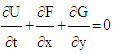(1)

In which: h: water depth, t: time, u: flow velocity in the x direction, v: flow velocity in the y direction, g: acceleration of gravity.

2.2. Site Studied and Data

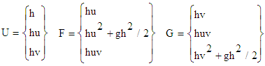
The study area is located in the northwestern part of Madagasca (Figure 1). The Sambirano River drains a 2.830 km² watershed with an average interannual rainfall, estimated at 2.500 mm. This information is listed in [8].

Figure 1. Global location of the studied site

In this area, for [5] the slope of the river is very low, which considerably increases the duration of the recession. The section we are interested in is special because of the existence of a bridge without piers to which the abutments considerably narrow the banks (Figure 2).

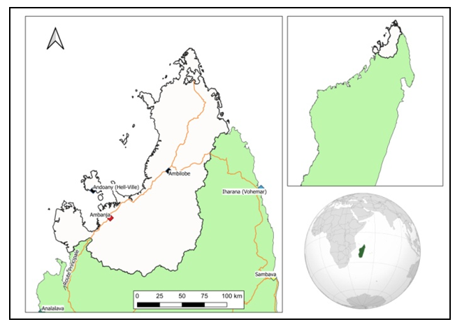
Figure 2. Topography and bathymetry of the section studied

One of the most important key elements in flood modeling is the hydrograph. It is recorded as a time series; however, it is not always available and especially in developing countries due to the lack of measured data according to [9]. For this purpose, a synthetic hydrograph based on the values indicated in [8] and shown in figure 3 for the condition at the entry.

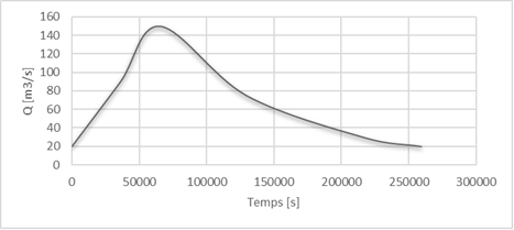Figure 3. Hydrograph at the entry of each model

2.3. Description of Numerical Methods and Software

The software we will be using are free solvers embedded in simple and popular graphical interfaces (Best Open source Software in Water Resources). Each solver is implemented for a real case, that is to say the same geometry. The solvers used are listed in table 1:

Table 1. Software (solvers) and the numerical method used

The figure 4 shows an overview of the methodology, data and adopted solvers.

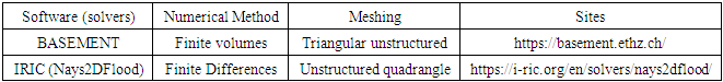
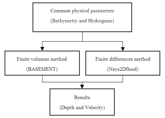Figure 4. Summary of the methods and software used

Referring to table 1 above each solver uses different meshes. The figure 5 shows each type of mesh.

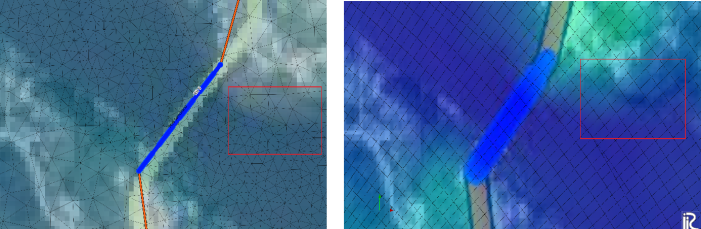Figure 5. Left: calculation grid for BASEMENT (unstructured triangular) and calculation grid for Nays2D flood (curvilinear quadrangle)

These illustrations (Figure 5) show the meshes under the Sambirano bridge. We can visualize in the red rectangle that the triangular mesh makes it possible to easily represent the curvatures of the banks, unlike the quadrangle mesh.

BASEMENT: The software is developed by the Laboratory of Hydraulics, Hydrology and Glaciology (VAW) of ETH Zurich. It is a hydro and morphodynamic model using finite volumes method solving the Shallow Water Equation system. The finite volume method consists of discretizing the flow domain into a multitude of control volumes, then performing mass and momentum balances on these small volumes. The advantage of the finite volume method lies in the fact that it ensures the conservation of mass, an important property to be respected by all calculations of fluid flows, and makes it possible to reduce an order of derivatives of the partial differential equations. The HLLC solver (Harten-Lax-van Leer-Contact) was developed by [10] in 1994. It restores the missing Rarefaction wave by some estimates, like linearizations, these can be simple but also more advanced, like using the average Roe speed for the average wave speed. For [11] They are quite robust and efficient but a little more diffusive.

NAYS2DFLOOD: It is a 2-dimensional flood analysis solver. It solves equations (1) and (2) using a curvilinear coordinate system and taking into account the coordinates adjusted to the limits by the finite difference method. The CIP method (Constrained Interpolation Pseudo-Particules or Cubic Interpolated Propagation), which is one of the options of the Nays2D Flood solver, was used for the resolution of the advection terms of the equations. It is a method which was first posed in 1985 by [12] and which subsequently underwent numerous developments, for example the method has been improved by [13] and [14].

2.4. Simulations Implementation

For the finite difference method, the simulation was carried out with the Nays2D Flood version 5.0 solver in the iRIC software suite version 2.3.9.6034 and with the following characteristics:

- A grid of 251 * 31 or 7781 meshes

- No calculation time Δt = 0.1

- Maximum number of iterations for the calculation of the surface: 10

- Minimum water depth: 0.20 m

For the finite volumes method we used BASEMENT 2.8 with the following characteristics:

- A grid of 17351 meshes

- A CFL condition of 0.8

- An exact type Riemann solver with an explicit scheme

- Minimum water depth: 0.20 m

3. Results and Discussions

The following figures show the depths of the flow at different times in the hydrograph. The images on the left relate to the results obtained using BASEMENT while the images on the right using IRIC, at the same time. The figures on the left show the water depths obtained with BASEMENT and those on the right by IRIC.

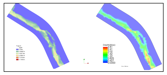Figure 6. Water depth in the domain at t = 7200s

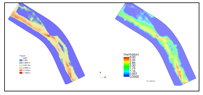Figure 7. Water depth at the peak of the hydrograph t = 80400s

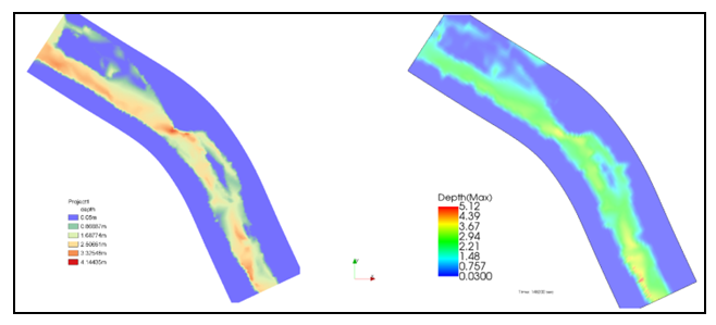Figure 8. Water depth during recession at t = 145200s

By analyzing figures 6, 7 and 8 we can draw the following lines:

- The results obtained generally reproduce reality (visual observation of a flood event) despite the lack of data available.

- The numerical results obtained with the two methods differ only very little.

Unlike the finite difference method which is a purely mathematical estimation, the first advantage of the finite volume method is based on the fact that it is based on the conservation law.

The two calculation codes are parallelizable, ie we can exploited the maximum number of threads possible for the computer hardware used. In this study, the source term modeling the precipitation that fell in the study area during the event is not considered. It can be considered in the digital diagram Nays2D flood unlike BASEMENT.

It can therefore be deduced that from a global point of view the two tools are reliable for modeling floods using a high resolution DEM.

Model validation

Lack of data on the study area prevented calibration and quantitative validation of the model. However, field investigations as well as the examination of various photos and videos during the flood have revealed an acceptable agreement between the results of the numerical simulation and the spatial extension that were actually produced in the area of studies. This qualitative calibration is a common process that has been carried out successfully around the world [15], [16], [17], [18] and [19] with the use of Nays2D Flood and BASEMENT because these solvers have been developed for developing countries where data is lacking [20].

4. Conclusions

Thanks to advances in the field of digital hydraulics, engineers and researchers are constantly improving the different methods and approaches in order to facilitate and get closer to reality in terms of modeling. This advance has given us the choice for interesting applications such as floods. The objective of this article was then to use the two usual numerical methods for solving flow equations in two-dimensional formulation in order to assess their relevance.

Simulation results have shown that both methods can be used for solving the Shallow Water Equation using a high resolution digital terrain model. For the two methods the implicit algorithm allows more important computation time steps than the explicit methods. For the finite difference method the mesh is not necessarily orthogonal but if the mesh is orthogonal the algorithm is simpler and more efficient. The finite volume method provides increased stability and improved robustness over traditional finite difference and finite element techniques.