John Weber1, George N. Facas2, Michael Horst3, Monica Sharobeam4
1Undergraduate Student, Department of Mechanical Engineering, The College of New Jersey, 2000 Pennington Road, Ewing, NJ
2Professor and Dean Emeritus, Department of Mechanical Engineering, The College of New Jersey, 2000 Pennington Road, Ewing, NJ
3Associate Professor and Chair, Department of Civil Engineering, The College of New Jersey, 2000 Pennington Road, Ewing, NJ
4Undergradaute Student, Department of Biomedical Engineering, The College of New Jersey, 2000 Pennington Road, Ewing, NJ
Correspondence to: Michael Horst, Associate Professor and Chair, Department of Civil Engineering, The College of New Jersey, 2000 Pennington Road, Ewing, NJ.
| Email: |  |
Copyright © 2019 The Author(s). Published by Scientific & Academic Publishing.
This work is licensed under the Creative Commons Attribution International License (CC BY).
http://creativecommons.org/licenses/by/4.0/

Abstract
Modeling software is becoming a valuable tool in undergraduate engineering education. Historically, computer programs were taught to students in design intensive courses, while introductory or fundamentals courses relied on the typical faculty led lecture format which was absent of any modeling applications or demonstrations. This trend is now changing as various engineering software packages are being introduced earlier in the curriculum as a tool to assist students in understanding the theory corresponding to a particular topic. This paper details the application of the FLUENT Finite Volume Modeling Software, in an introductory fluid mechanics course, to a segment of pipe which experiences a sudden contraction. Students were able to explore various fluid phenomenon including: the development of fully developed flow, the linear relationship between pressure drop and distance, minor loss coefficients as a function of contraction ratio, and visualization of the contracting flow field. Qualitative feedback from students has shown appreciation for being introduced to modern engineering tools that are used in the practice of engineering.
Keywords:
Teaching, Fluid Mechanics, FLUENT
Cite this paper: John Weber, George N. Facas, Michael Horst, Monica Sharobeam, Using FLUENT to Supplement Theory in an Introductory Fluid Mechanics Course, International Journal of Hydraulic Engineering, Vol. 8 No. 1, 2019, pp. 11-21. doi: 10.5923/j.ijhe.20190801.03.
1. Introduction
Numerical modeling of fluid flow is becoming increasingly popular. Computing power coupled with user friendly software interfaces have made model development and execution practical at the undergraduate level. Historically, obtaining solutions to complicated fluid dynamics problems has been limited to primarily experimental work and secondarily closed form solutions of the governing theoretical equations. Now with commercially available Computational Fluid Dynamics (CFD) software packages, high accuracy solutions to complicated fluid dynamics problems can be obtained. Systems can be parametrically studied in three dimensions (3D) using finite element/difference/volume techniques, once the CFD model has been validated with either theoretical or experimental data. In a typical introductory (undergraduate) fluid mechanics course students are presented with the Navier Stokes Equations. A series of assumptions then are applied which ultimately lead to the development of the 1D Bernoulli Equation. Students learn the principles of the Bernoulli Equation in idealized situations and then expand upon it by incorporating both major and minor energy losses (i.e. – the Energy Equation). When introducing the energy loss terms, an analytic derivation is used to develop an equation for friction losses for laminar flow, while dimensional analysis is used to develop the Darcy equation for turbulent flow. Comparison of the two equations allows for the Darcy friction factor under laminar flow conditions to be determined. The Darcy friction factor under turbulent flow conditions was determined empirically and is shown graphically in the Moody Diagram. Additionally, when considering minor losses, empirical coefficients and graphs are used to determine expected energy losses due to changes in system geometry or obstructions encountered by the flow. It should be noted that the typical graphs used to determine minor loss coefficients for certain geometric changes (expansions and contractions for pipes in series) are based on turbulent flow conditions. Loss coefficients for laminar flow conditions often are omitted in standard textbooks developed for civil and mechanical engineering students and therefore a full analysis of the system dynamics is not possible for these groups of students without using other resources such as CFD models. While the use of software modeling has typically been reserved for graduate level and undergraduate senior-level design intensive engineering courses, its integration into the introductory or mechanics courses is proving to be beneficial (Collins & Bhaskaran, 2003) (Sert & Nakigoblu, 2007) (Daneshfaraz, et. al., 2018). Students not only are being introduced to the models earlier in their academic careers which ultimately will lead to a greater understanding of the full potential of certain software packages for design applications, they also are able to use these models as a means to cross validate numerical solutions to empirically derived coefficients found in most mechanics and fundamentals courses such as a first level fluid mechanics course.An assignment was given in an introductory fluid mechanics course where students were asked to develop a CFD model using FLUENT in order to identify flow characteristics under laminar flow conditions in a pipe with a sudden contraction. Students worked in teams of two and each group of students were asked to evaluate the system under different flow conditions (both Reynolds numbers and pipe ratio diameters). The students were expected to go through the entire CFD model development process from solid model generation, to grid meshing, to specifying boundary conditions and selecting a solution method, to experimenting with convergence criteria and obtaining a reasonable grid-independent converged solution, to post-processing and interpreting the numerical results, and finally to benchmarking the solution to data given in the literature. The goals for the assignment included: allowing students to understand how easily the model could be developed, and giving the students an understanding of the changing flow dynamics as the flow enters the pipe, passes through the sudden contraction and then continues through the smaller pipe. Additionally, students were able to acquire the following information and compare it to theoretical and empirical expectations: developing region of the velocity profile as the distribution goes from uniform to parabolic, verification that the friction factor under laminar fully-developed flow conditions equals sixty four divided by the Reynolds number, the relationship between the contraction minor loss coefficient and the ratio of the pipe diameters, the identification of the vena-contracta region and how it relates to the minor losses, and stream-line visualization for the purpose of qualitatively understanding the flow characteristics near the contracted section. The following sections detail the model development and present results for each of the topics listed above. The sections are presented in a sequential order as the flow moves from upstream to downstream within the pipe. At the completion of the assignment a discussion ensued with the students which focused on the underlying theory and the ability of CFD models to produce reasonably accurate solutions to complex fluid dynamics problems.
2. Finite Volume Model
ANSYS Fluent finite volume software was used to simulate laminar flow of water at 20°C through a pipe with a sudden contraction. Several geometries were created, using varying ratios of the cross-sectional areas of the downstream to upstream sections, Ad/AD, from 0.1 to 0.9. The geometry was positioned within a Cartesian coordinate system, with the centerline of the pipe lying along the x-axis, the contraction occurring at x=0, and the flow occurring in the positive x-direction as shown in Figure 1. For all the simulations, an upstream diameter (D) of 12.7 mm and an upstream length (L) of 100 times the diameter was used. To determine an appropriate downstream length (l), a number of downstream diameters (d) was calculated by the students based on a convention of 0.06 times the downstream Reynolds number (Red) plus twenty additional diameters, to ensure the flow would return to a fully developed state after passing through the sudden contraction.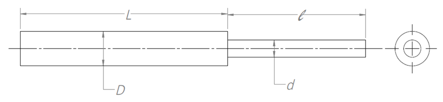 | Figure 1. Sketch of the Sudden Contraction Geometry |
To reduce the computational effort and time required for each simulation, only one quarter of the interior of the pipe was meshed and simulated, using symmetry boundary conditions in the XY and XZ planes. The grid mesh was generated using a hex-dominant method and hexahedral elements with a size of 0.3 mm. An element size of 0.3 mm was found to yield solutions which were independent of element-size for all Reynold’s numbers and area aspect ratios considered. A typical grid mesh generated by Fluent is shown in Fig 2. Figs 2a and 2b show different views of the grid mesh near the sudden contraction. Fig 2c shows a perspective view of the grid mesh at the exit plane of the pipe. For each Fluent simulation, a uniform velocity boundary condition was applied at the inlet of the pipe while a pressure boundary condition of 0 Pa (gage pressure) was applied to the outlet. A no-slip boundary condition was also applied to the wall of the pipe. The coupled pressure-velocity method along with second order upwind scheme for the momentum was used (instructed to use) for solving the governing equations. Each simulation was set to iterate until the residuals for continuity of x-, y, and z-velocity all reached below 1x10⁻⁴. For these residuals, convergence was achieved in approximately 125 iterations.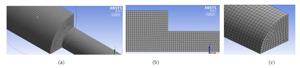 | Figure 2. Typical grid mesh generated by Fluent, d/D = 2 |
Hydrodynamic Developing Region Downstream of the Entrance to a Tube.The hydrodynamic developing region is the region downstream of the tube entrance where an axisymmetric boundary is growing at the walls of the tube and nearly an inviscid core flow exists at the center of the tube, as shown schematically in Fig. 3. For laminar flow, the accepted correlation for the developing length Le is (Pritchard and Mitchell, 2015).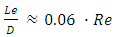 | (1) |
where ReD is the Reynolds number.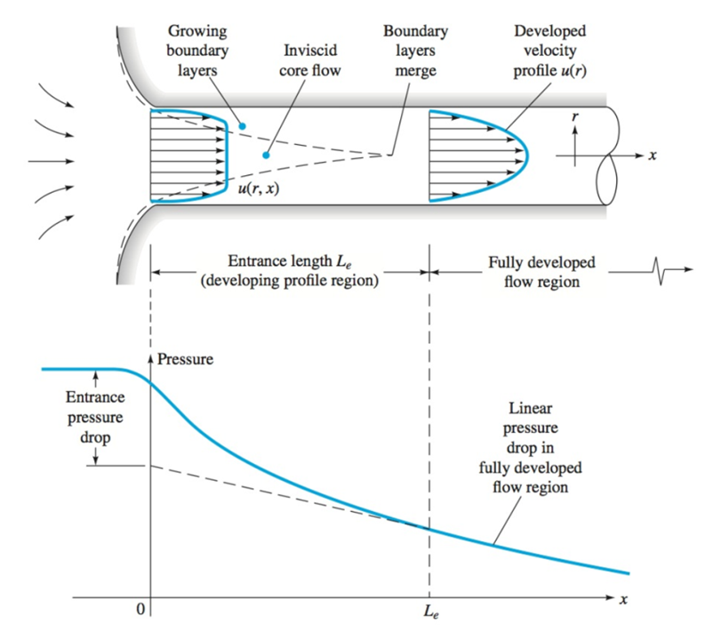 | Figure 3. Axial velocity profiles and pressure drop in the developing region of pipe flow |
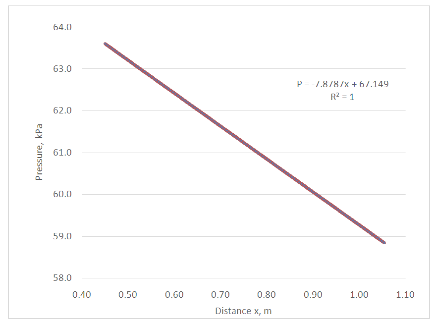
Sample Finite Volume Analysis (FVA) solutions for the axial velocity profiles at various distances from the tube entrance obtained in the current study are shown for ReD equal 200 and 500 in Figs. 4 and 5 respectively. The charts illustrate the effect of the growing viscous boundary layer in terms of a reduction of the axial velocity near the wall and an inviscid core fluid flow. At a finite distance x = Le from the entrance, the inviscid flow has disappeared, the flow has become entirely viscous, and the axial velocity no longer changes with x. At this point the flow is considered to be fully developed. Downstream of x = Le, the velocity profile does not change, the wall shear is constant, and the pressure decreases linearly with x, as will be demonstrated later. 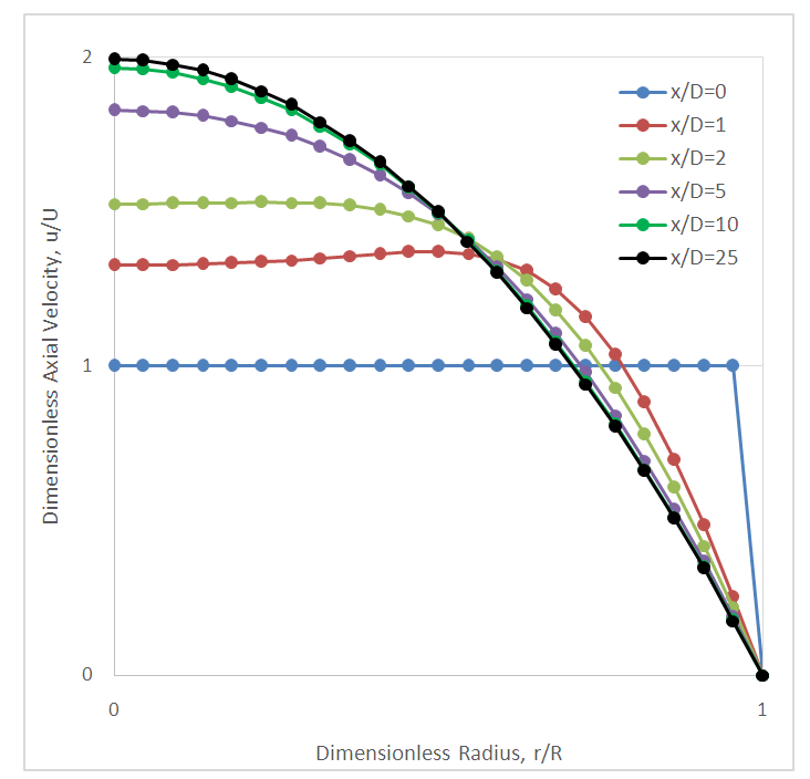 | Figure 4. Dimensionless axial velocity profiles downstream of the tube entrance (x/D), ReD = 200 |
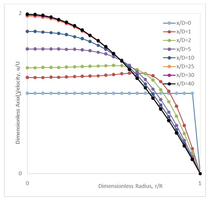 | Figure 5. Dimensionless axial velocity profiles downstream of the tube entrance (x/D), ReD = 500 |
Clearly, the prediction for the developing region length Le is in great agreement with the accepted correlation given by Eq. (1). Based on these results the students were able to visualize the changing velocity profile as it transitioned from uniform to parabolic.After analyzing the changing velocity profile, discussion was shifted to focus on how the pressure within the system varies as a function of distance along the pipe. Sample FVA solutions for the pressure drop as a function of distance from the tube entrance are shown in Figs. 6 and 7. The results from the FVA analysis were compared to results presented by Shah and London (1978) which were obtained from the finite difference numerical solutions presented by Hornbeck (1964) for laminar flow in the entrance region of a pipe. It is interesting to note that near the pipe entrance the pressure drop is not linear which is due to the changing velocity profile. It is only after the velocity distribution becomes parabolic and constant (i.e., fully-developed flow) that the pressure drop becomes linear with distance. 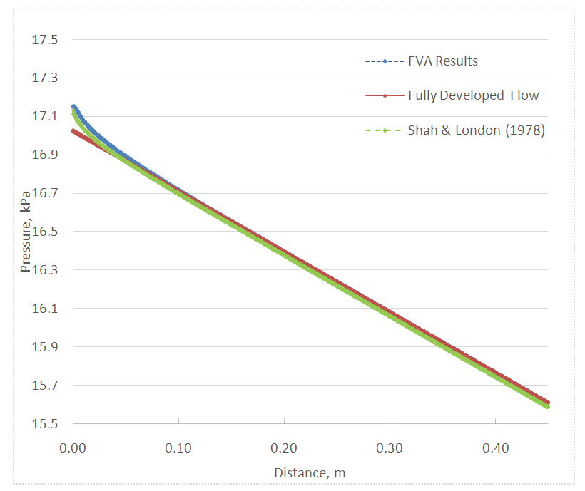 | Figure 6. Pressure drop downstream of the tube entrance, ReD = 200 |
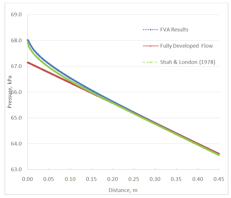 | Figure 7. Pressure drop downstream of the tube entrance, ReD = 500 |
The pressure drop in the fully developed region is usually expressed in terms of the Darcy friction factor. | (2) |
where f is known as the Darcy friction factor and for laminar flow is given by | (3) |
∆p = Pressure Drop (Pa)L = Length (m)D = Pipe diameter (m)g = Gravity (m/s2)U = Average velocity (m/s)For laminar flow in the fully developed region, the wall shear is constant and, therefore, the pressure drops linearly with distance. Sample pressure drop FVA results as a function of distance for laminar flow in the fully developed region are shown in Figs. 8 and 9 corresponding to ReD =200 and ReD=500 respectively. Also shown in Figs 8 and 9 are the results of linear regression best fit correlations for the pressure as a function of x. These correlations were used to calculate the equivalent Darcy friction factor that the FVA solution yields. Assuming that the friction factor  it can be shown that the constant β can be calculated using Eq. (4) where m is the slope of the linear correlation shown in Figs. 8 and 9.
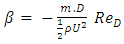 | (4) |
For the sample FVA results shown in Figs 8 and 9, the values calculated for β are 64.01 and 64.05 respectively which are in excellent agreement with the closed form solution of β=64 for laminar pipe flow and any differences may be attributed to numerical round-off or truncation error within the solution algorithm.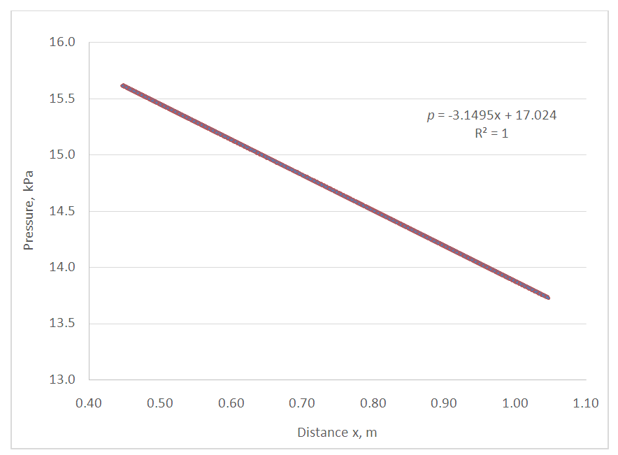 | Figure 8. Pressure drop in the fully developed region in a tube. ReD = 200 |
 | Figure 9. Pressure drop in the fully developed region in a tube. ReD = 500 |
As the fluid flow approaches the sudden contraction, the flow pattern is affected by it. Sample dimensionless axial velocity profiles upstream of the sudden contraction are shown in Fig. 10. These profiles are similar to the finite difference solutions presented by Durst and Loy (1985). The FVA results shown in Fig. 10 indicate that the axial velocity profile remained parabolic up to 1 diameter “D” upstream of the sudden contraction. Downstream of the sudden contraction, the flow redevelops in agreement with the accepted correlation given by Eq. (1) into a parabolic profile, as is illustrated in Fig. 11. | Figure 10. Dimensionless axial velocity profiles upstream of the sudden contraction (x/D), ReD = 500, AR=0.25 |
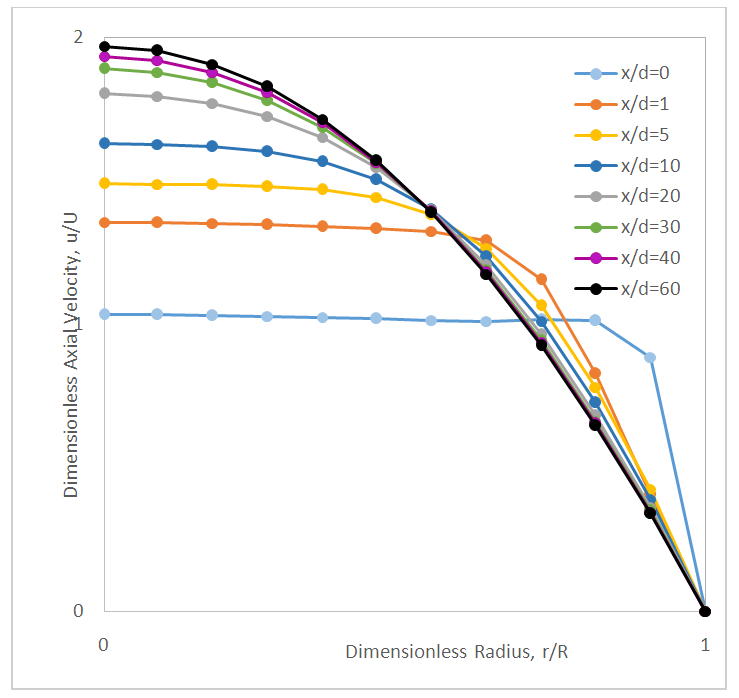 | Figure 11. Dimensionless axial velocity profiles downstream of the sudden contraction (x/d), ReD = 500, AR=0.25 |
3. Fluid Flow through a Sudden Contraction
When the fluid passes through a sudden contraction, a loss in pressure occurs. Holmes (1967) proposed Eq. (5) for determining the pressure drop that occurs across the contraction.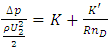 | (5) |
where U2 is the average velocity downstream of the contraction and K and  are often referred to as the Hagenbach and Couette correction coefficients, respectively. Kaye and Rosen (1971) experimentally determined that the dependence of K and K’ on the aspect area ratio
  is given for Newtonian fluids by the following two expressions.
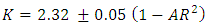 | (6) |
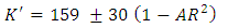 | (7) |
The pressure drop  across the sudden contraction in these FVA simulations was determined using Eq. (8) where p1 and p2 are the pressures at two points far upstream and far downstream of the sudden contraction, respectively, and where the assumption of fully-developed flow was valid at both points.
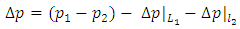 | (8) |
The terms  and
and  represent the pressure drop due to friction for fully developed-flow over a distance L1 upstream of the contraction and a distance
  downstream of the contraction corresponding to the distance to point 1 and 2 from the sudden contraction, respectively. Eq. (3) was used in calculating the terms
  and
and  Sample FVA solutions for the dimensionless pressure drop as a function of aspect ratio AR and ReD are shown in Fig. 12. The best fit correlation results of Kaye and Rosen (Eq. (6) and (7)) are also shown in Fig. 12 for ReD = 500. Clearly, the FVA results for the dimensionless pressure drop do not indicate any dependence on ReD. Moreover, the FVA results obtained in this study are lower than those that are predicted using the best fit correlation of Kaye and Rosen. This finding is, however, consistent with the findings of Durst and Loy (1985) which are also lower than the experimental data of Kaye and Rosen. The difference between the FVA results and the best fit correlation of Kaye and Rosen varies from 5 - 35% with the largest difference corresponding to the lower ReD number.
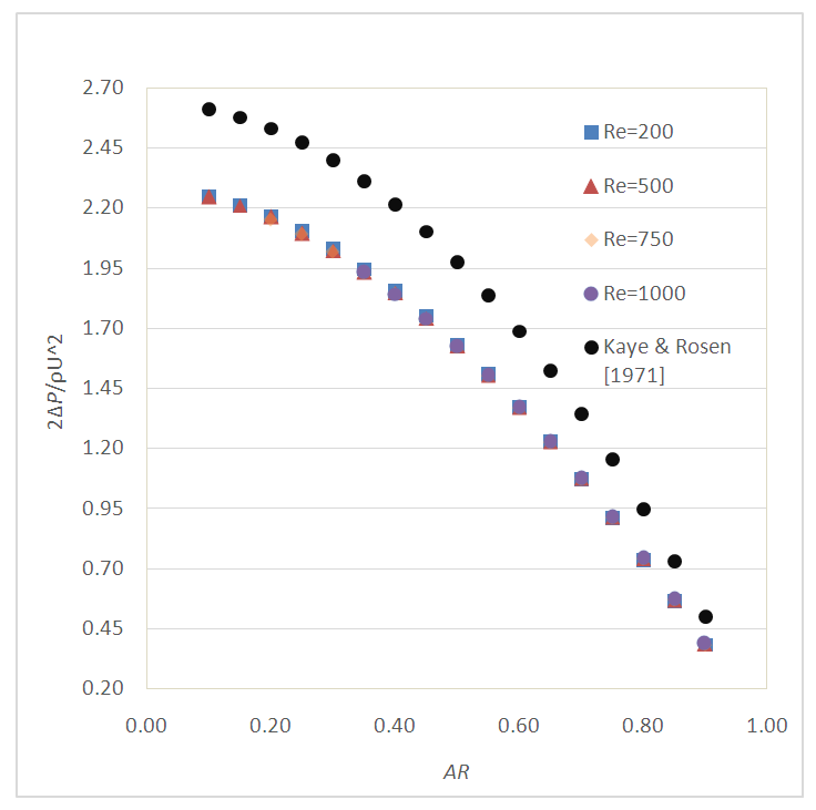 | Figure 12. Dimensionless pressure drop across a sudden contraction. Kay and Rosen data shown correspond to ReD = 500 |
4. Energy Considerations in Pipe Flow
The energy equation for one-dimensional incompressible fluid flow in a horizontal pipe is usually written as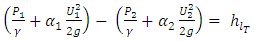 | (9) |
where  represents the total energy loss per unit mass,
  is the fluids specific weight, and p1 and p2 static pressure.
  and
and  are referred to as the kinetic energy coefficients. For fully developed laminar flow,
 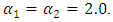 The total energy loss,
  consists of major losses (friction losses) and minor losses. Minor losses are encountered across fittings, bends, or abrupt area changes and occur primarily because of flow separation. In the case of laminar, fully-developed flow in a pipe of constant diameter, major losses,
  can be calculated using Eqs. (2) and (3). Minor losses,
  are usually expressed in terms of a loss coefficient,
 | (10) |
The minor loss coefficient,  , across the sudden contraction can therefore be calculated using the pressure prediction at point 1 upstream of the contraction and point 2 downstream of the contraction with both points being far away from the contraction such that fully-developed flow can be assumed to exist at both points. Thus,
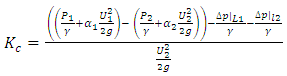 | (11) |
where  and
and  represent the pressure drop due to friction (major losses) for fully developed-flow over a distance L1 upstream of the contraction and a distance l2 downstream of the contraction corresponding to the distance to point 1 and 2 from the sudden contraction, respectively. It can also be shown that for laminar fully developed flow the relationship between the minor loss coefficient, KC, and the Hagenbach and Couette correction coefficients is given by Eq. (12).
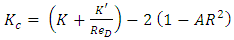 | (12) |
Sample FVA solutions for the minor loss coefficient, KC, as a function of aspect ratio AR and ReD are shown for laminar flow in Fig. 13. The FVA results for KC are lower than typical KC data presented for fluid flow through a sudden contraction by many Fluid Mechanics textbooks, e.g. see Pritchard and Mitchell (2015) where values typically range between 0.0-0.5. The reason for the discrepancy is due to the fact that typical relationships presented in standard textbooks are based on turbulent flow whereas the results of these simulations are all for laminar flow. This particular learning outcome was not anticipated and further amplified the benefits of using FVA modeling software as a tool to aid undergraduate students in comprehending fluid flow phenomena.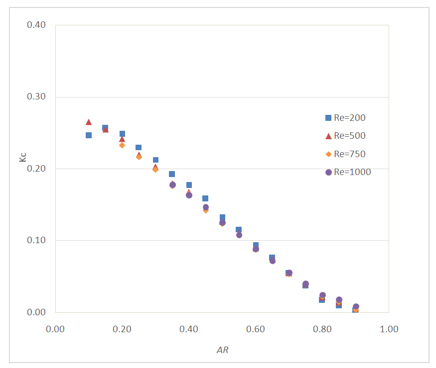 | Figure 13. Minor loss coefficient across a sudden contraction |
The final benefit of using FVA software for studying fluid flow phenomenon is the ability of Fluent to plot fluid flow streamlines and, hence, qualitatively study the resulting fluid flow pattern. A typical streamline plot near the sudden contraction generated with FLUENT is shown in Fig. 14, which clearly demonstrated the concept of a vena-contracta downstream of the sudden contraction and further reinforced that the numerical solution of the theoretical equations produced results which are qualitatively in agreement with theoretical and/or experimental images found in standard fluid mechanics textbooks. Students were able to see not only the affect that the contraction has on the corresponding flow conditions but also visualize additional flow characteristics such as the presence of a secondary (vortex) fluid flow.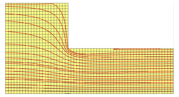 | Figure 14. Typical streamline plot for fluid flow in a pipe network with a sudden contraction |
5. Assessment of Student Learning and Conclusions
The integration of this activity into a required introductory fluid mechanics course is proving to be very beneficial to the overall understanding of fluid mechanics for students. The numerical simulation of laminar fluid flow in a pipe network with a sudden contraction has provided an opportunity for students to deepen their understanding of key fluid mechanics concepts such as: fully-developed fluid flow; fluid flow in the developing region; major and minor energy losses; and fluid flow visualization. Although student performance in terms of completing the assignment and presenting results and conclusions has varied from excellent to poor, students have, in general, shown great appreciation for being introduced to modern engineering tools that are used in the practice of engineering. Here is how one student commented in an anonymous end of semester class evaluation survey which was completed online: “The Fluent assignment, while challenging, was an excellent project especially since it was our first time being introduced to the software.” A second student said: “I enjoyed diving into the theory behind the fluent pipe flow simulation.” There has been no negative comments submitted about this assignment on the online end of semester class evaluation survey. In addition, a significant number of students have informally expressed their satisfaction to the class instructors as well as other faculty members for the opportunity given to them to work and experiment with an industry-standard software package during the junior year. As a consequence of this opportunity, more students have been observed to have used Fluent in their Senior Design Project over the last two years as compared to prior years when no assignment of this type was assigned in the basic fluid mechanics course. One of the lessons learned is that, in order for the students to successfully complete all phases of the assignment, they must be given ample amount of time to work on it. As a result, the assignment must be given relatively early in the semester. Solid model construction and volume grid generation could be given before any of the fundamental concepts have been presented to the students. Moreover, the assignment must be broken into weekly smaller student deliverable modules starting with the solid model construction and volume grid generation followed by comparing solutions for various grid sizes and convergence criteria to which input must be continuously provided by the instructor before they can proceed to the next phase of data analysis and interpretation as well as report submission. In general, students seemed to be overwhelmed initially but with enough feedback and support the majority of students were able to successfully complete all phases of the project. Faculty (or teaching assistants) availability to answer questions is critical to students’ ability in successfully completing the project. Hence, class size must be held small if no teaching assistance is available to the instructor.
References
| [1] | Collins, L., Bhaskaran, R., 2003, Integration of Simulation into the Undergraduate Fluid Mechanics Curriculum Using Fluent, ASEE, paper presented at the 2003 Annual Conference, Nashville, TN. |
| [2] | Daneshfaraz, R., Rezazadehjoudi, A., Abraham, J., 2018, Numerical Investigation on the Effect of Sudden Contraction on Flow Behavior in a 90-Degree Bend, KSCE Journal of Civil Engineering, Vol. 22 (2), p 603-612. |
| [3] | Durst, F., Loy, T., 1985. Investigations of Laminar Flow in a Pipe with Sudden Contraction of Cross Sectional Area. Computers & Fluids, vol. 13, No. 1, pp. 15-36. |
| [4] | Holmes, D. B., 1967, Dissertation, Delft. |
| [5] | Hornbeck, R. W., 1964. Laminar Flow in the Entrance Region of a Pipe. Appl. Sci. Res., 13, 224-232. |
| [6] | Kaye, S. E. and Rosen, S. E., 1971, AIChE J., 17, pp. 1269-1270. |
| [7] | Pritchard, P. J. and Mitchell, J. W., 2015, Fox and McDonald’s Introduction to Fluid Mechanics, 9th Ed, Wiley. |
| [8] | Sert, C., Nakigoblu, G., 2007, AC2007-1560: Use of Computational Fluid Dynamics (CFD) in Teaching Fluid Mechanics, ASEE, paper no. AC 2007-1560, 2007. |
| [9] | Shah, R.K, London, A.L., 1978. Laminar Flow Forced Convection in Ducts. Supplement I to Advances in Heat Transfer, Academic Press, New York, NY. |

 Abstract
 Reference
 Full-Text PDF
 Full-text HTML