1. Introduction

River morphology entails geometric and physical properties of rivers, such as topography and bed shape and their interaction with flow characteristics, such as velocity and flow resistance and is therefore important in predicting river behavior. The role of bed forms in river banks was investigated by Gilbert (1914). The resistance to flow depends on bed form and its roughness. Beds have different forms, depending on the flow and type of river, including pools and riffles. In this study the velocity distribution in the outer region was investigated over artificial riffles were investigated, considering the variation of Coles parameter and von Karman constant. The gravel and sand particles make up the, generating the bed forms studies very attractive in fluvial hydraulics. The effect of non-uniform flow on the turbulent flow structure has attracted much attention, because in normal currents a uniform flow is rarely observed, and bed-forms, lateral contractions, and vegetation are often caused by non-uniform flow (Afzalimehr et al. 2017). The non-uniform flow can be summed up in two groups of accelerating and decelerating flows. The streaming current is a flow with a positive pressure gradient and a flowing stream current is with a negative pressure gradient. The equilibrium flow is a stream independent of its upstream conditions, in which the distributions of velocity and turbulence components are also shaped. In the boundary layer theory, the flow in open channels can be distinguished into two regions-inner and outer. 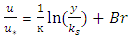In the inner region, which is limited to in uniform flow, the velocity profile can be expressed by the wall law as equation (1). The wall law states that the average velocity of a turbulent stream is proportional to a logarithmic distance from that point to the wall. This law was considered by von Karman (1930), which particularly applies to a portion of the current near the bed (less than 20% of the depth of the stream).

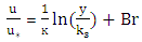(1)

In this equation, u is the mean point velocity at depth is shear velocity, k is Von Karman's constant, is the roughness scale and Br is the integral constant.

In coarse bed rivers the boundary layer thickness develops up to the water surface, dividing the boundary layer into two separate regions: The first region is close to the bed, where there is significant viscosity, and is called the inner region. As one moves away from the river bed in the vertical direction, the effect of turbulence increases and the viscosity decreases and this state continues to the water surface. This part is referred to as the depth of the outer layer (Schlichting 1979), where the first law for the velocity distribution was provided by Bazin as follows:

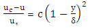(2)

In this equation, is the maximum velocity, u is the velocity of the point at the distance y from bed. the shear velocity, c is a constant coefficient, and δ is the depth of the boundary layer.

The above parabolic rule is for the outer region of velocity profile but does not apply to the inner region.

In the outer region, velocity data diverges from the wall law. The amount of deviation can be determined by the wake function, first proposed by Coles (1956). The point at which velocity data diverges from the logarithmic law depends on the maximum velocity, the thickness of boundary layer, and the pressure gradient. Nezu and Rodi (1986) applied the wake law to uniform flow on a smooth base and the developed a logarithmic law as follows:

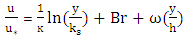(3)

where the wake function was defined as:

(4)

In this regard, Π is the Coles parameter that depends on the Reynolds number and the pressure gradient. Equation (4) can be rewritten as equation (5), which can be used both in the inner and outer regions and on flat and rough substrates:

(5)

is the maximum velocity occurring at δ = y.

A study of bed forms involves Froude number, Reynolds number, average velocity, shear velocity, shear stress, and friction coefficient representing the entire bed form. The equilibrium flow is a stream that does not depend on its past and can be used to reach overall results for uniform flows. In non-uniform flow, the depth and flow velocity vary from one location to another, and observations of equilibrium flow can be used to determine the characteristics of a general flow cross section representing all sections of a channel. The velocity profiles alone cannot indicate an equilibrium boundary layer in which the velocity profile and turbulence profiles, such as must remain coincident at different sections in the channel, where , are the values of velocity fluctuations in the longitudinal and vertical directions. Using the dimensionless pressure gradient, Clauser (1954, 1956) proposed:

(6)

Where is the displacement thickness of boundary layer.

If β does not change for velocity profiles in the direction of flow, then flow is equilibrium.

The literature review in the subject reveals that few study is prevalent on the effect of convex bed forms (riffles) on the velocity distribution, validation of Coles parameter in the outer region and variation von Karman constant. The objective of this study is to investigate the validation of Coles parameter, the parabolic law and von Karman constant over an artificial riffle.

2. Experimental Setup and Measurements

Data for this study were collected in a rectangular channel, 8 meters long, 40 cm wide, and 60 cm high in the hydrological laboratory of the Faculty of Agriculture of Isfahan University of Technology. The bottom of channel and its walls were made of glass and the slope of the floor was changed using a lever under the channel.

The water from the tank was pumped into the inlet pipe by a centrifugal pump with a maximum flow rate of 50 liters per second. The water discharge was measured through a digital flow-meter installed on the inlet pipe of the canal. The depth of water was measured by a depth-measuring device that had Ashley with a precision of 0.01 cm and was transported on the upper rails of the canal in two directions: longitudinal and transverse. Fig. 1 shows a view of the laboratory flume.

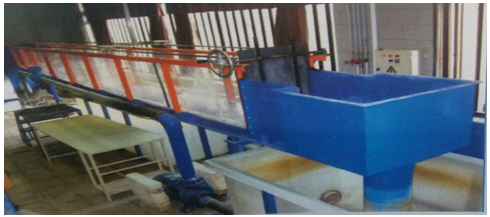Figure 1. View of the laboratory flume in this research

Three-dimensional water velocity measurements were made using the ADV velocity-meter. This device used the Doppler effect to measure flow velocity by sending a short pulse and listening to its echo, and then measuring the pitch variations or reverberation frequency.

The device used in this study is the Nortek Series Vectrino + model, which has a sampling frequency of up to 200 hz (Gil Montero et al. 2014). The purpose of this study was to investigate flow on riffles. On the other hand, the particle diameter was chosen in such a way that their threshold of motion was greater than flow velocity. Granular particles with a diameter of were selected to compare with other studies on bed forms (Nasiri et al. 2011, Fazlollahi et al. 2015, Kabiri et al. 2015).

In field surveys of Zayandeh-rood River in Isfahan, the shape of riffles in the Zayandeh-rood River, which is classified as a gravel river, is generally with a grain size of . For this reason, the shape of riffles was investigated in experiments with .

In order to simulate riffles in the laboratory channel, the Carling et al. (1914) data were used in the third part of the Ciuron River. The average width of the river was 43.58 meters and the length of the projection was 163.71 meters. It was reported that the dimensions were simulated in a laboratory with a widths of 40 cm and a 15 cm riffle length at scale of 1:10000. This length of bed form was completely located in the area from the beginning of channel and the area that was far from the effect of the end of valve and in this regard was the most suitable bed-form for this channel. According to Carling's observations, the angle of input and output in this form of bed was only a few degrees, usually less than 6 degrees. Therefore, the angle of 5 degrees was selected as the angle in the laboratory.

The bed forms 5.1 meters in length were made at a distance of 5 meters from the beginning of the channel with the help of wooden molds. The flow rate was selected to achieve the desired depth by adjusting the end of valve by trial and error of such that the depth of water was 20cm and there was no movement of particles. A digital flow-meter with a precision of was installed on the channel entrance pipe, which adjusted discharge. A quasi-uniform flow was obtained by measuring the flow depth along the channel.

Velocity profiles were measured at 10, 20, 30, 40, 60, 80, 100, 110, 120, 130, 140, 150, and 160 cm along the riffle. These profiles at the channel center are named a, b, c, d, e, f, g, h, i, j, k, l, and m, respectively (Fig. 2). The shear velocity was determined by the Clauser method and the boundary layer specification was also used for the parabolic method.

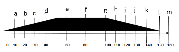Figure 2. Schematic of the simulated bed form in laboratory

All data measured by ADV were filtered by using WinADV software as described above, and then velocity and turbulence parameters on each flow path were calculated and analyzed. The WinADV software has the ability to analyze and process data measured by ADV.

The Coles parameter is obtained using graphical and analytical methods. This parameter reflects the deviation of velocity profile from the logarithmic law in the outer region; it was estimated in this study graphically and analytically. For the graphical method the velocity values were obtained by plotting the values of against log on a semi-log paper. After linearly fitting to the external region data, the velocity profile and its extension along the vertical axis to a point at which the value was , were obtained. From this value, which was equal to , the value of the Coles parameter was obtained. Fig. 3 shows the estimation of Coles parameter.

Kironoto used an analytical method to calculate Π using the following relation:

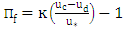(7)

where is the mean velocity depth defined as:

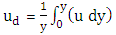(8)

Figure 3. Estimation of the Coles parameter

3. Analysis of Results

3.1. Application of Wake Law and Comparison with Parabolic Law on a Riffle

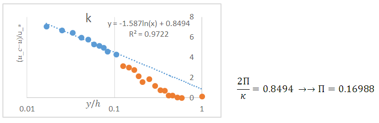
As shown in Fig. 4, the Coles law represented the data in the outer region.

Fig. 5 shows Coles parameter by both graphical and analytical methods (Table 1). Considering similar variations on the length of the bed, it can be said that the Coles empirical law for smooth and sloping bed without forms can be generalized for riffles.

The difference between graphical and analytical methods is the hypothesis and the geometric bed form, as shown in Fig. 5. It seems that the assumption was not valid for riffles. Also, the thickness of the inner region of the inner and outer layers had a significant effect on the bed form and the change in its geometry in the estimation of the boundary layer. The ineffectiveness of the assumptions led to different results by analytical and graphical methods.

Fig. 6 shows the validity of parabolic law in the outer region, which shows the deviation of this rule in the inner layer for 6 velocity profiles at different points on the bed. The parabolic of law, as Coles law, perfectly fitted the data of the inner and outer regions.

Figure 4. Velocity distribution in the outer region fitted by Coles law on the riffle. Figs. a, b show accelerating flow and Figs. f, g show quasi-uniform flow and j, k show decelerating flow

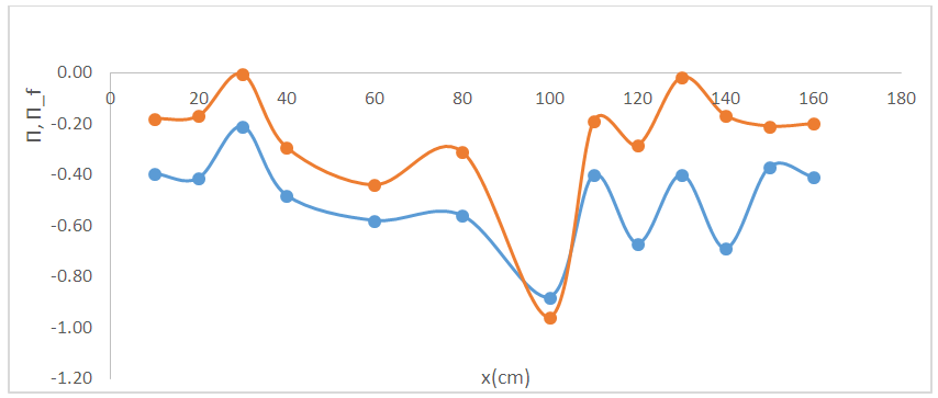Figure 5. Comparison of Coles parameter on riffle (red series: calculated Coles parameter by graphical method and blue series: calculated Coles parameter by analytical method) along the bed

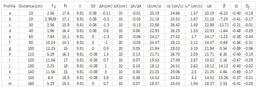Table 1. Calculation of β and the Coles parameter by analytical method Π and graphical method Πf

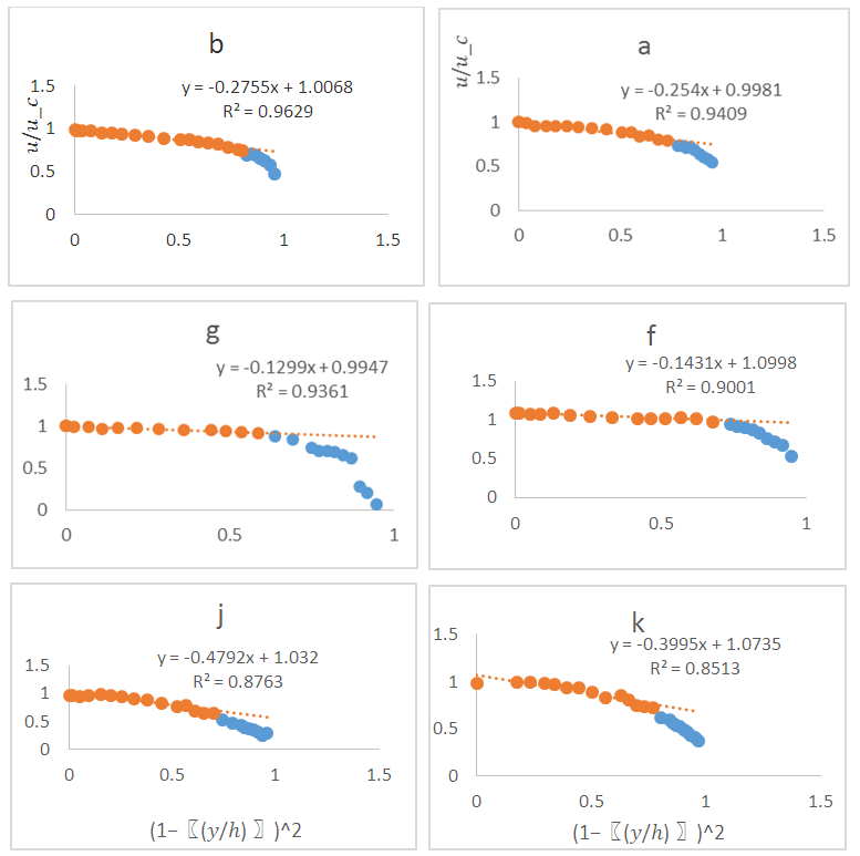Figure 6. Fitness of parabolic law to velocity data on the riffle. Figs a, b show accelerating flow, Figs f, g show quasi-uniform flow and Figs. j, k show decorating flow

3.2. Relationship between the Coles Parameter Π and the Dimensionless Pressure Gradient β

The pressure gradient parameter was defined as follows (Graf and Altinkar, 1998):

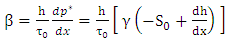(9)

which was used to parameterize non-uniform flow. For uniform flow . (In the open channel, based on equation (9), (Kironoto 1991).

Here, the pressure gradient parameter was defined as:

where is the free flow velocity (maximum flow velocity in the velocity profile), and θ, are the displacement and the momentum thickness of boundary layers, respectively, defined as:

(10)

(11)

For a boundary layer with a pressure gradient of zero, the value of Coles parameter was Π≃0.5, while for uniform flow, due to the effect of roughness of the negative-pressure gradient stream, the average value of Π was 0.09 (White, 2007). For equilibrium flow (where the velocity distribution and turbulence components along the longitudinal were similar), the values of Π remained constant. The relationship between the value of Π during non-uniform stresses and the pressure gradient parameter Π=f(β), has been considered in the literature. Kironoto has shown that the Coles parameter depends on the pressure gradient parameter, and the relationship between them is governed by non-uniform and uniform flow channels. Using non-uniform flow data, with fitting by regression of the Coles parameter against the pressure gradient parameter, Kironoto obtained the following relation:

(12)

Using the available data, the values of Π were calculated graphically and analytically for 13 profiles. Also, the pressure gradient parameter for each profile was also calculated. In all profiles throughout the bed form, there was no strong correlation between the pressure gradient parameter and the Coles parameter, but in the accelerating section of the flow on the riffle, according to Fig. 7 Coles parameter obtained from two different methods had a significant correlation with the gradient pressure parameter. Equations (13) and (14) express correlations between the Coles parameter (computational and graphical) and pressure gradient:

(13)

(14)

Figure 7. Relation between Coles parameter and pressure gradient parameter: A and B-Calculation of the Coles parameter by graphical method. C and D-Calculation of the Coles parameter by analytical method

3.3. Determination of the von Karman Constant κ

Von Karman's constant is important for calculating velocity and shear velocity by logarithmic and parabolic laws. To determine Π by regression, the fitted regression line was extrapolated to internal data to cut the horizontal axis from the curve , and the resulting value was equal to . In order to more accurately calculate the Coles parameter, it was necessary to calculate the von Karman constant coefficient for the riffle.

To calculate the constant von karman of the logarithmic law and the application of velocity profiles related to the 13 sections of the central axis of the channel and regressing u versus :

(16)

By fitting the logarithmic law equation to the data of the inner region of boundary layer, the slope and width of the origin are respectively.

The von Karman constant was calculated for the 13 velocity profiles, as presented in table 2.

Table 2 show that the calculated von Karman constant from the shear velocity by the boundary layer method was closer to the global constant 0.4 and showed less fluctuations for the bed than by other methods.

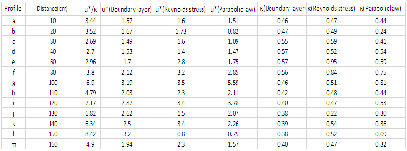Table 2. The values of (von Karman constant) by using different methods

4. Conclusions

The boundary layer flow in gravel bed on the riffle is distinguishable in the inner and outer regions. In the inner region, the logarithmic law was established, and the data deviation from the logarithmic law of velocity in the outer region of the boundary layer , where z is the distance from the bed and h, the depth of the flow, was used to explain the deviation of data from the inner region of the rule (function wake).

Calculations showed that the outer part of the boundary layer was represented well by a parabolic law, but the inner region of the boundary layer did not follow this rule. To determine the relationship between the Coles parameter Π and the dimensionless pressure gradient β, the first step was calculated using a pressure gradient equation for 13 velocity distribution profiles. Then, the Coles parameter was calculated using theoretical and graphical methods. The correlation between the pressure gradient parameter and the Coles parameter obtained from the two methods for the total data showed a very low correlation coefficient. Using velocity data and shear velocity data obtained from boundary layer characteristics method, Reynolds stress, parabolic law, and logarithm law, von Karman constant was calculated. Comparison of results showed that the von Karman constant obtained by the boundary layer characteristics method was closer to the universal constant value of 0.4.

To calculate the Coles parameter, von Karman's constant was used.

Notation