1. Introduction

Velocity distributions in open channel flows are required for a wide range of hydraulic applications relating to sediment transport, river pollution, channel scouring and power plant design. Therefore, the velocity profile, in particular over the vertical, has been given a great interest by many researchers. Beside numerous investigations, which have been conducted to measure the turbulent mean velocity profiles, theoretical laws are formulated, and hydrodynamic models are constructed for obtaining the velocity distributions to both the 2D and 3D flow cases.

When 2D open channel flows are being considered, the well-known logarithmic law proposed by Keulegan [1] and Nikuradse [2] is widely used for obtaining the velocity profile in the inner region (z < 0.2h), where z is the vertical distance from the bed and h is the flow depth. However, the log law was reported to deviate from the experimental data in the outer region (z > 0.2h), [3, 4]. This deviation was first addressed by Coles [3] by adding the wake function to the log law. The log-wake law was found to be more accepted than the conventional log law for describing the velocity profile in wide open channels, provided that the wake strength parameter to be set to an empirically determined value, [4, 5].

However, in case of narrow open channel flows, the log-wake law deviates from the experimental data near the free surface. This is because such a law cannot be able to capture the velocity-dip-phenomenon, which causes the maximum velocity to occur below the water surface. The velocity-dip-phenomenon occur due to strong secondary currents generated in three-dimensional open channel flow [6]. Therefore, several analytical and semi-analytical equations have been proposed, trying to predict the velocity-dip-phenomenon in open channels by accounting for the effect of the secondary currents. Almost, all the analytical-based laws proposed are based on the analysis and simplification of the Reynolds-averaged Navier-Stokes equations (RANS).

Yang et al. [7] proposed a dip-modified-log law (DML-law) using simplified RANS formulations. Although the DML-law is able to predict the velocity dip position, this law was derived to predict the velocity profile in only smooth channels with some limitations about specifying the position of the maximum velocity. Thus, many researchers have continued to offer improvements to both the log and wake laws for smooth or rough flows [8-12]. Based on the same simplification of RANS equation used by Yang [7], but with using the log wake formulation instead, Absi [11] proposed another law for velocity, called dip-modified-log-wake law (DMLW-law). This modified law can be used in a smooth and rough open channel flow with the secondary currents because of its ability to predict the velocity dip, [13]. Lassabatere et al. [12] developed a simplified model by integrating the RANS equations through proposing a number of hypotheses, focusing in particular on the analytical analysis for the velocity vertical component. Despite the advantage of these laws in terms of easily applying to engineering problems, they all are based on proposed assumptions for the secondary velocities and eddy viscosity to simplify the RANS equations before the integration. Therefore, many researchers have discussed the validity of such laws, e.g. [12, 14, 15]. It was found that the assumptions employed in simplifying the RANS equation when deriving the dip-modified laws are still needed a further check. Thus, in this paper, the proposed dip-modified laws for velocity distribution is compared with three dimensional models which are based on the full RANS equations. The Computational Fluid Dynamics (CFD) technique was used to solve the full RANS equations. By comparing the results from the simplified RANS formulations (dip-modified laws) with those from the full RANS model (CFD model), the errors result from the former can be estimated. This may assist in determining the limitations of the dip-modified laws for engineering applications.

2. Simplified RANS Approaches

2.1. Basic Equations and Assumptions

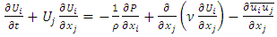
As mentioned previously, dip-modified log formulations were generally derived from RANS equations by simplifying these equations. This simplification can be made by imposing some assumptions to account for the effect of the secondary currents (normal wall or vertical component of velocity) and by using an appropriate expression for the turbulent eddy viscosity.

For steady uniform open-channel flows, the continuity equation and the RANS momentum equation in the streamwise direction (x) can be combined to give the following equation (Figure 1):

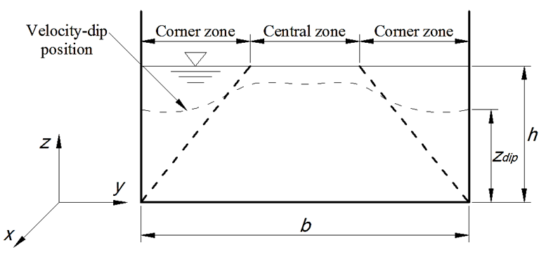Figure 1. Definition sketch for the steady uniform flow in a rectangular channel

(1)

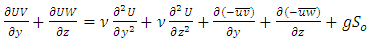
where and are mean velocity in the streamwise (x), lateral (y), and vertical (z) directions, respectively; is gravitational acceleration; is channel slope; and are Reynolds stress tensor components; and ν is fluid kinematic viscosity of fluid. In the central zone (Figure 1), it is assumed that the horizontal gradients (d/dy) are negligible comparing to the vertical gradients (d/dz) which are dominating in this zone, [7]. Therefore, Eq. (1) can be simplified to:

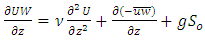(2)

After integration and algebraic manipulations, the following equation is obtained:

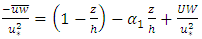(3)

where is the friction velocity, h is the flow depth and

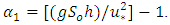In most simplified RANS approaches, two additional assumptions were often imposed on Eq. (3). One for modelling the Reynolds shear stress and the other for approximating the secondary flow term The third term on the right-hand side of Eq. (3), which reflects the influence of secondary currents, are often approximated using a linear relationship for simplicity, [7]:

(4)

where is a positive coefficient. On the other hand, the Boussinesq assumption are frequently used to model the Reynolds shear stress as following:

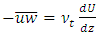(5)

where is the eddy viscosity. Substituting Eq. (4) and Eq. (5) into Eq. (3), the following partial differential equation (PDE) is obtained:

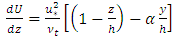(6)

Equation (6) is the simplified form of RANS equations which is used as a basic equation for deriving the dip modified laws to obtain the mean velocity profile of the uniform flow. Depending upon the models by which the eddy viscosity is expressed, different formulations for calculating the velocity distribution can be obtained from the simplified RANS equation, Eq. (6).

2.2. Dip-modified Laws

2.2.1. Dip-modified Log Law (DML-law)

Yang et al. [7] employed the parabolic model for the eddy viscosity to suggest DML-law based on Eq. (6). The widely used expression of the parabolic model is:

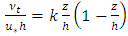(7)

where k is the so-called Von Karman constant. Using Eq. (7) into Eq. (6) and making the integration, the final form of the DML-law can be obtained:

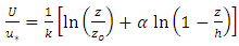(8)

where is the distance from the bed at which the velocity is hypothetically equal to zero and is he dip-correction parameter. Equation (8) predicts the velocity-dip phenomenon by the term 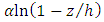which includes the dip-correction parameter [7]. This law returns into the classical log law if

2.2.2. Dip-modified Log Wake Law (DMLW-law)

Instead of the parabolic model, the approximation for the eddy viscosity distribution given by Nezu and Rodi [4] can also be employed in the simplified RANS Equation, Eq. (6), to drive a dip modified law for the velocity distribution [11]. Nezu and Rodi [4] suggested their model for eddy viscosity based on the log-wake law and it can be written as:

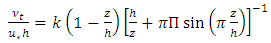(9)

where is Coles parameter representing the wake strength in the boundary turbulent flow. If the eddy viscosity model given by Nezu and Rodi [4], Eq. (9), is used instead of the parabolic profile, the integration and simplification of Eq. (6) would yield the following dip-modified log wake law (DMLW-law):

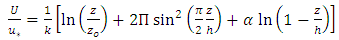(10)

This law is also called the dip-modified log wake law (DMLW-law).

There are more complicated forms for the dip-modified laws such as Total DMLW-law proposed by Absi [11] and the model presented by Lassabatere et al. [12]. However, compromising between the simplicity in use of the less complicated model and a little improvement in accuracy obtained by the more complicated one makes using the simplest formulation of dip-modified laws in engineering applications more convenient. Therefore, in this study, the performance of dip-modified log law, Eq. (8), and the dip-modified wake law, Eq. (10), are only compared as a simplified RANs approaches against the 3D full RANs model that is solved using the CFD technique.

3. 3D Full RANS Modelling

3.1. Mathematical Framework of the CFD

In this study, ANSYS CFX 13.0 code was used for performing the 3D CFD modelling. In this software, the Reynolds Averaged Navier-Stokes (RANS) equations are used to simulate the 3D turbulent flow in an open channel. The RANS equations are obtained by applying time averaging to the full Navier-Stokes equations. For an incompressible and turbulent fluid flow, RANS equations may be written in a Cartesian coordinate system as follows:

(11)

(12)

where the subscripts i, j (= 1, 2, 3) refer to the components in the x; y and z of the Cartesian coordinate system, U is the mean velocity, P is the mean pressure, and u is the velocity fluctuation. The Reynolds-averaging of the Navier-Stokes equations introduced six new unknowns into the governing equations. These extra unknown quantities comprise the so-called Reynolds stresses. Hence, a turbulence model is then required to account for the Reynolds stresses in order to close the system of equations.

3.2. Turbulence Model

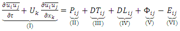
Various turbulence models have been developed to solve the closure problem of RANS equations. These models relate the Reynolds stresses to the global mean properties of the fluid flow on a physical basis. In general, two closure strategies are typically used to develop practical turbulence models for engineering computations, [16, 17]. The first strategy is the eddy-viscosity concept, whereas the second modelling strategy relies on directly solving transport equations for the individual Reynolds stresses.

It is found that the models based on eddy viscosity concept, such as k-ε model and k-ω model, fail to predict any evidence of secondary flow in a prismatic channel such as the cases investigated in this work. This is due to the assumption that the turbulence is isotropic, but in such channel, the turbulence is actually known to be anisotropic, [18; 19]. Therefore, the models falling under this category were not employed for conducting 3D simulations during this study. On the contrary to the eddy viscosity-based models, Reynolds Stress models (RSM) physically include the effects of streamline curvature, sudden changes in the strain rate, anisotropic Reynolds stress and secondary flows, [20, 21]. Based on this fact, a Reynolds stress model (RSM) may be more appropriate for flows with secondary flows. Therefore, BSL RSM turbulence model which is falling under this category has been implemented in this study.

BSL RSM is based on the Reynolds stress transport equations. The exact transport equation for the Reynolds stresses in Cartesian tensor notation is as follows [22]:

(13)

where is the production of the turbulence, is the turbulent diffusion due to the fluctuations, is the diffusion of the Reynolds stresses due to molecular mixing, is the pressure-strain redistribution term and is the viscous dissipation of Reynolds stresses. Terms (I), (II) and (IV) contain only mean velocity components and the Reynolds stresses, thus, they do not require modelling when Eq. (13) is used to close the mean flow Eq. (12). On the other hand, terms (III), (V) and (VI) introduce 22 new unknowns into the governing equations, thus they need to be modelled to close the equations.

The modelled form of exact transport equation for the Reynolds stresses are written in the CFX as follows, [23]:

(14)

The pressure-strain is modeled within CFX by the following constitutive relation:

(15)

in which, is the specific dissipation rate, is the unit tensor (Kronecker’s delta) and is the mean rate of strain tensor. The production tensor of Reynolds stresses is given by:

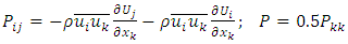(16)

The tensor is given by:

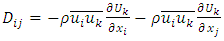(17)

The coefficients for the model are:

(18)

It should be referred that the BSL RSM is based on the BSL k-ω model of Menter [24]. Menter’s model blends between k-ω the model near the wall and the k-ε model in the outer region by the following equation:

(19)

where blending function F takes a value of 1 near the wall and decreases to a value of zero outside the boundary layer [24].

4. Applying the Models

4.1. Experimental Data Used

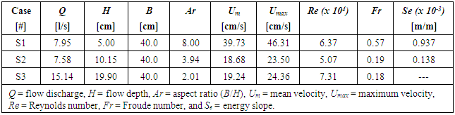
The velocity results from dip-modified laws, which are based on the simplified RANS approaches, and those predicted by CFD model, which is based on the full RANS equations, were both compared with experimental data to test their performance in predicting the velocity distribution. The data obtained from the experiments conducted by Tominaga & Ezaki [25] and Tominaga et al. [26] were used for this purpose. The first group in these experiments, which included the experiments on a smooth rectangular channel, only was considered herein.

The channel used had a length of 12.5 m, width of 40 cm and height of 40 cm. Experimental conditions for flow cases in this group are given in Table 1. The channel width was fixed in all the three cases (S1, S2 and S3), whereas the flow depth was changed. Therefore, selecting these experiments will allow examining the effect of the aspect ratio and the secondary currents on the performance of the model tested.

Table 1. Experimental conditions for the rectangular smooth channel used by Tominaga & Ezaki [25] and Tominaga et al. [26]

4.2. Applying Simplified RANS Models

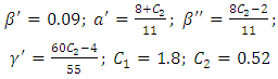
As presented in previous section, the DML-law (Eq. 8) and the DMLW-law (Eq. 10), take the velocity-dip phenomenon into consideration by using the dip-correction parameter Therefore, should be first estimated before application of the models.

An empirical formula, which is proposed by Yang et al. [7], could be used for finding This formula relates the dip-correction parameter to (z/h) and is given as:

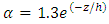(20)

However, it was found that the computed velocity profile may not match well with the experimental data when is calculated by using Eq. (20), [9, 13, 27]. Absi [11] proposed another relation for calculating the dip-correction parameter:

(21)

where is normalized distance of maximum velocity measured from the channel bed. In the central zone, Yan et al. found that depends closely on the aspect ratio (A_r), and decreases with the increase of A_r, [7]. Equation (21) produces results consistent well with this fact. Hence, in this study, Eq. (21) was employed to estimate the value of in both simplified RANS models (i.e. DML-law and DMLW-law).

Added to the estimation of the dip-correction parameter, the wake strength parameter (Π) also need to be estimated when the DMLW-law is applied. Π seems to be not universal and its value depends on turbulence structure and the effect of secondary currents. Cebeci and Smith found experimentally that Π increases with Reynolds number in zero-pressure-gradient boundary layers, and at high Reynolds numbers, Π rises to a value of 0.55, [28]. Nezu and Rodi indicated through Laser Doppler anemometry velocity measurements that Π increases significantly with the Reynolds number but becomes nearly constant (Π ≈ 0.2) for 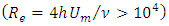, where is the mean bulk velocity [4]. Cardoso et al. observed in their experiments on smooth open channel that a wake of small strength (Π ≈ 0.08) occurred in the core of the outer region (0.2 < z/h < 0.7), followed by the retarding effect near the free surface due to the downflow of the secondary currents [5]. This suggests that the secondary currents may influence the wake strength and cause the value of Π to be lower.

The flow cases considered in this study are almost narrow channels (except S3) and have a relatively high Reynolds number, therefore the effect of the secondary currents at the center of the flow is considerable. Therefore, a value in a range from 0.0 to 0.2 could be selected for the wake strength parameter. However, in all velocity calculations conducted by the dip-modified laws herein, it was found that the agreement between computed and experimental results was rather better when Π takes a value of 0.2. Hence, the value of Π = 0.2 was used for all test cases considered in the present work.

4.3. Applying 3D CFD Simulations

A computational CFD model was built by the commercial code (CFX 13.0) to simulate the cases S1, S2 and S3 of the experiments by Tominaga et al. [26]. This means, three different aspect ratios were considered, i.e. (A_r = 8.0, 3.94 and 2.01) as shown in Table 1. Figure 2 shows the computational setup and the boundary surfaces for the flow cases simulated herein.

Figure 2. Schematic of domain geometry and boundary conditions

The width and height of the computational domain were chosen to be similar to those of the corresponding experimental flume. But, the domain length of 0.1 m has been used for the geometry under consideration. Since the flow is uniform and can be assumed to be statistically homogeneous in the streamwise direction, the periodic boundary conditions with a constant pressure gradient (Δp) were applied. This allowed for the solution domain to be setup with a much shorter length and fewer cells in streamwise direction than using a longer length required for establishing the fully developed flow, [29, 30].

In all simulations conducted in this study, the free-slip condition with the modified free surface treatment supplied by CFX was imposed on the free surface boundary. Through this approach, the turbulence terms at the free surface are modified in a similar way as in the approach proposed by Celik & Rodi [31] to mimic the damping of turbulent fluctuations by the surface. Using this modified boundary condition helps to reproduce the effect of the velocity dip by reducing the turbulent length scale near a free surface [29]. For the channel walls (bed and side walls), the smooth no-slip wall boundary conditions were imposed for all test cases simulated in the present study.

Throughout this work, hexahedral cells have been utilized and this has been relatively easy to implement with the non-complex geometries being considered. To ensure that the mesh adopted is sufficiently fine so that it does not affect the results, a mesh independence study was performed first. Based on the mesh independence study, all results predicted were obtained using the mesh sizes of Δx = 2.5mm, Δy = 2.0 mm and Δz = 2.0 mm.

For all simulations conducted in this study, the reliable convergence was considered to be achieved when the root mean square (RMS) residual of main variables in mass and momentum equations dropped below the residual target value (1 x 10^-6). In addition, flow rate and average streamwise velocity were also monitored and used as additional convergence criteria. The monitoring points specified within the CFX had to reach nearly constant values and equal to those from experiments in order for the simulation was assumed to be met all convergence criteria.

5. Results and Discussion

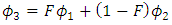
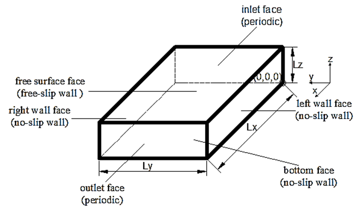
To evaluate the performance of the simplified RANS model, i.e. DML-law or DMLW-law, against the full RANS (CFD) model, the results predicted by both models were compared with the measured data.

Figure 3 compares the velocity profiles computed by the conventional log law, DML-law and 3D CFD model with experimental data from Tominaga et al. [29] for the three flow cases considered (S1, S2 and S3). It should be pointed out here that the log law was included in the comparison, due to the reason that this law represents the case where the dip correction factor in DML-law is reduced to the zero. The results show that both the full RANS (CFD) model and the simplified RANS (DML-law) model are able to simulate the velocity dip, with the CFD reproducing the velocity profile more accurately. Although the dip-modified-log law (DML-law) can predict the dip phenomenon well, a noticeable deviation between its results and the experimental data can be seen. This deviation is thought to be associated with the assumptions for approximating the effects of the secondary currents and eddy viscosity. As discussed earlier, to derive the DML-law from the simplified RANS equation, Eq. (6), the vertical velocity (W) in the outer region is assumed to be in the downward direction over all the centre of the channel and the eddy viscosity was modelled without considering the wake strength effect. This means that an exaggerated value of the dip modified term is applied to the entire flow depth, resulting in the underestimation of predicted velocities. It is also clear from the Figure 3 that DML-law can represent the measured velocity profile more closely when the dip correction factor is set to be zero (i.e. DML-law turns into log law). Nevertheless, it is not possible to predict the velocity dip feature by using the log law (or DML-law with of zero). Thus, DML-law may not be able to predict the maximum velocity location and, at the same time, lead to accurate computations of the velocity profile by only adjusting the factor .

Figure 3. Mean streamwise velocity profile, comparing the simplified RANS model (DML-law) and full RANS model (3D CFD model) with the experimental data from Tominaga et al. [26]

Figure 4 shows the comparison between the velocity profiles computed by the simplified RANS (DMLW-law) and the full RANS (CFD) model with that obtained experimentally by the Tominaga et al. [26]. The velocity profiles from the log wake law were also plotted in the figure to represent the application of the DMLW-law with neglecting the dip correction factor. From the figure, it is noted that the velocity profile predicted by DMLW-law is nearly close to the flume measurements and highly close to the full RANS predictions for all test cases, except a slight difference for the case S3. This indicates that the DMLW-law may predict the velocity distribution in the same order of the accuracy of the full RANS based model, and also more accurate than the DML-law. Therefore, it is suggested that including the wake strength parameter (Π) into the simplified RANS model improve the predicted results. Figures 3 and 4 shows that the CFD results for the velocity are more accurate compared with both the simplified RANS models used in the present study. This is not surprising because the CFD model is based on the full RANS equations. However, it should be noted that the ability of the CFD model with RSM turbulence model to predict the dip velocity phenomena is not typical. 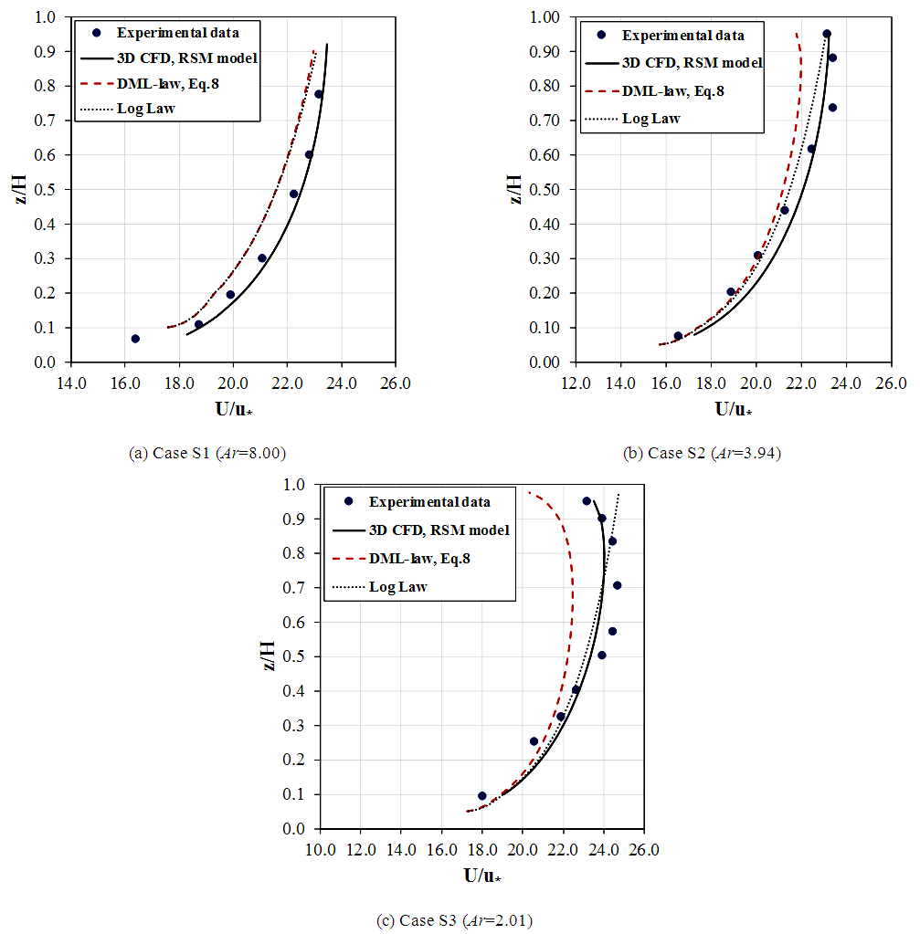This is suggested to be a consequence of the underestimation in the turbulence anisotropy of the normal stresses as shown in Figure 5. Although a modified treatment for the free surface boundary conditions are used, the magnitude of the computed turbulence anisotropy at free surface zone (z/h > 0.7) is comparatively low with respect to the measured data. This may affect predicting the secondary velocity components (V, W) which are responsible for generating the velocity dip. To improve the predicted results from the full RANS (CFD) model, more sophisticated boundary condition is required to impose at the free surface. This makes the application of the full RANS model more impractical for engineering problems compared to using the simplified RANS-based models.

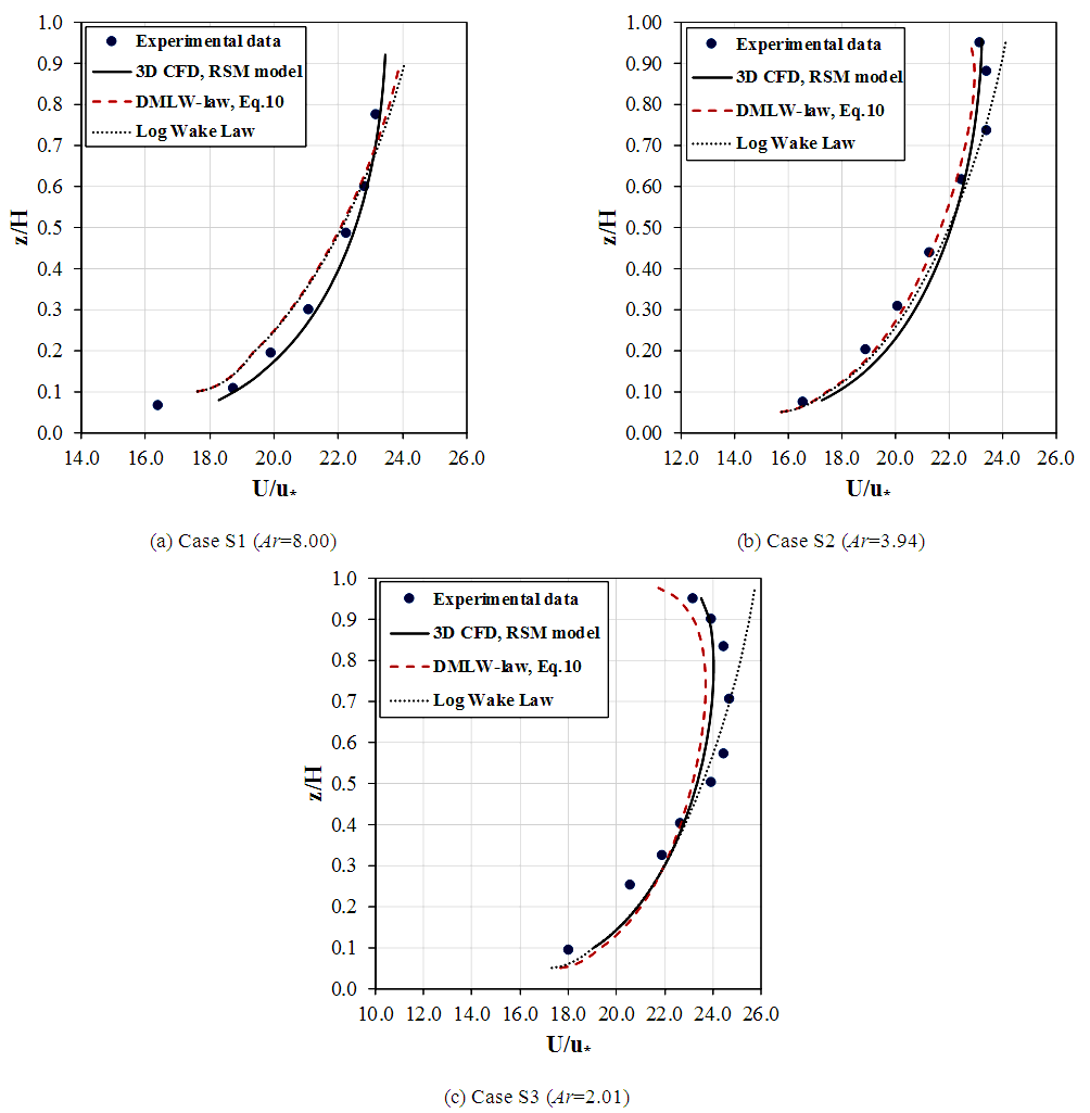Figure 4. Mean streamwise velocity profile, comparing the simplified RANS model (DMLW-law) and full RANS model (3D CFD model) with the Experimental data from Tominaga et al. [26]

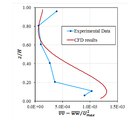Figure 5. Turbulence anisotropy of the normal stresses for case S3 at the channel centre: computed by CFD model and measured by Tominaga & Ezaki [25]

To quantitatively evaluate the performance of the simplified RANS models and compare them with that of the full RANS CFD model, the root-mean-square deviation (RMSD) is given as an index for comparison:

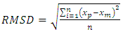(22)

where , are predicted and measured values respectively, and n is the total number of data in each of the individual profiles.

The RMSD of for all models used and for all test cases are summarized and shown by the bar-graph in Figure 6. It can be seen that the 3D CFD models based on full RANS equations gives nearly the lowest values of RMSD (0.3, 0.4, and 0.6), compared to those obtained for both dip modified formulations based on the simplified RANS equations. However, the DMLW-law, which include the wake effect, may give velocity results with RMSD values (0.5, 0.6 and 0.9) close to those for full RANS model. DML-law gives the greatest RMSD of 1.8 for the case S3 (i.e. for the narrowest channel) while DMLW-law improves the prediction with RMSD of 0.9. Additionally, Figure 6 shows that the velocity profiles computed by conventional log wake law deviate from those measured with RMSD being less or equal to that obtained for DML-law.

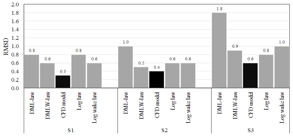Figure 6. Root mean square deviation (RMSD) for predicted velocity from measured data

6. Conclusions

The performance of the dip modified laws, which are based on the simplified RANS equations, are tested against the application of the full RANS model used in the CFD modelling. The results for velocity profiles obtained by two simplified RANS models, namely dip-modified log law (DML-law) and dip-modified log wake law (DMLW-law), and by the full RANS (CFD) model are compared with the experiments conducted by Tominaga et al. [26] for uniform flow in a smooth rectangular channel. Form comparison and analysis of the predicted velocity profiles obtained by all the models, it can be concluded that:

1) The dip-modified log law (DML-law) given by Eq. (8) is able to capture the velocity dip phenomenon but it underestimates the predicted velocity in the outer region, particularly for the narrowest channel.

2) The dip-modified log wake law (DMLW-law) is able to predict the dip velocity and can give a better prediction for velocity than the DML-law due to including the wake effect on the velocity. However, the performance of DMLW-law is still less than the full RANS model.

3) The full RANS (CFD) model predicts the velocity profile with a high degree of accuracy if compared with the both dip modified laws. However, the CFD modelling cannot predict the velocity dip phenomenon perfectly even though a complicated turbulence model with complicated formulations for boundary conditions are used. Therefore, it would be impractically difficult to use the full RANS model for velocity calculations in engineering applications.

4) The underestimations of the predicted velocity by DML-law are suggested to be due to the assumption of the secondary currents effect and the negligence the wake effect.

5) Based on the root mean square deviation (RMSD), which is calculated for all the models in the interest, the DML-law gives the least accurate results for the velocity, while the DMLW-law can give results close to the full RANS model (CFD).