Thair Sharif Kayyun, Dheyaa Hamdan Dagher
Building and Construction Engineering Department, University of Technology, Baghdad, Iraq
Correspondence to: Dheyaa Hamdan Dagher, Building and Construction Engineering Department, University of Technology, Baghdad, Iraq.
| Email: |  |
Copyright © 2018 The Author(s). Published by Scientific & Academic Publishing.
This work is licensed under the Creative Commons Attribution International License (CC BY).
http://creativecommons.org/licenses/by/4.0/

Abstract
The length of the reach river for the study area is (19.5 Km) lies in Northern of Tigris river between Al- Muthana bridge and Sarai gauging station in Baghdad city in Iraq. HEC-RAS version (5.03) was employed by making use of recorded field measurements data for running, calibration and verification processes. A new equation for the rating curve was introduced to estimate the water surface elevation at the upstream and downstream of the river reach. This rating curve was created by using four flow rate scenarios (461, 890, 1815 and 2500 m3/s) in which water surface elevation ranging between 26.67 and 33.45 (m.a.s.l). For sediment transport analysis Laursen (Copeland) formula showed a good agreement with the measured field data. Changes in the river bed have been studied for the period from 2012 to 2017. The depth of erosion and sedimentation were calculated at the upstream and downstream of the river reach which are equal to 0.51 and 0.39 m, respectively. The cumulative average depth of the erosion of the river bed for the future period from 2017 to 2040 was estimated to be about 1 m for discharge of (461 m3/s).
Keywords:
Tigris river, HEC-RAS version (5.03), Sediment transport, Depth of erosion and sedimentation
Cite this paper: Thair Sharif Kayyun, Dheyaa Hamdan Dagher, Potential Sediment within a Reach in Tigris River, International Journal of Hydraulic Engineering, Vol. 7 No. 2, 2018, pp. 22-32. doi: 10.5923/j.ijhe.20180702.02.
1. Introduction
The Tigris River is one of the most important rivers in the Middle East. It rises from the Taurus Mountain range in the southeastern part of Turkey and flows towards the southeast for 1580 km, passing through Turkish-Syrian borders and entering Iraq. In Iraq, it flows towards the south until it combines with the Euphrates River at Qurnah, forming the Shatt Al-Arab River. This river discharges its water into the Arabian Gulf. Within Baghdad City, the capital of Iraq, the Tigris River bisects Baghdad into two parts for a distance of about 50 km within the urban zone starting. The first reach of the Tigris river (19.5 Km length) lies at Northern reach of Tigris river between Al- Muthana Bridge and Sarai gauging station. The second part ending at the confluence with the Diyala River to the south. This river reach has single thread, compound meanders, and alluvial plain characteristics. Sediment transport rates are highly affected in the course of the Tigris river upstream of Baghdad due to the trapping of sediment within the reservoirs of dams upstream of Baghdad, [3], [8] conducted a training study of Tigris River for the benefit of Iraqi Ministry of Irrigation to improve the river flow conditions and the usage of the banks. They conducted a land and bathymetric surveys for a reach of 59 km of Tigris River within Baghdad City. They established an equation for the suspended sediment discharge with respect to water discharge. They used six formula of bed load sediment discharge to predict it and they proposed a band of bed load discharges with respect to water discharge instead of preferring a single formula. The estimated bed load discharge was between 1600-4300 m3/day for the mean annually water discharge (1035 m3/s) while the estimated suspended load discharge was 8500 m3/day. These values were considered “high” for the suspended load and “important” for the bed load sediment. The annually total sediment discharge was estimated as 11 million tons for the mean hydrological year. [17] conducted a training study for the Tigris River in Baghdad similar to the study of [8]. They considered two bathymetric surveys conducted in 1988 and 1991. A 2-D morphological model was applied to determine the velocity distribution and water surface profile that can be used to specify the locations of river banks that require protection, and specified the types of protection to be considered, as well as specifying depositional zones and the formation of islands.
2. Study Area
The selected reach of the Tigris river (19.5 Km length) lies at Northern reach of Tigris River between Al- Muthana Bridge and Sarai gauging station in Baghdad city in Iraq. Figure 1: A and B. This area was selected because it has no tributaries and there are a few structures that intersect with the selected reach.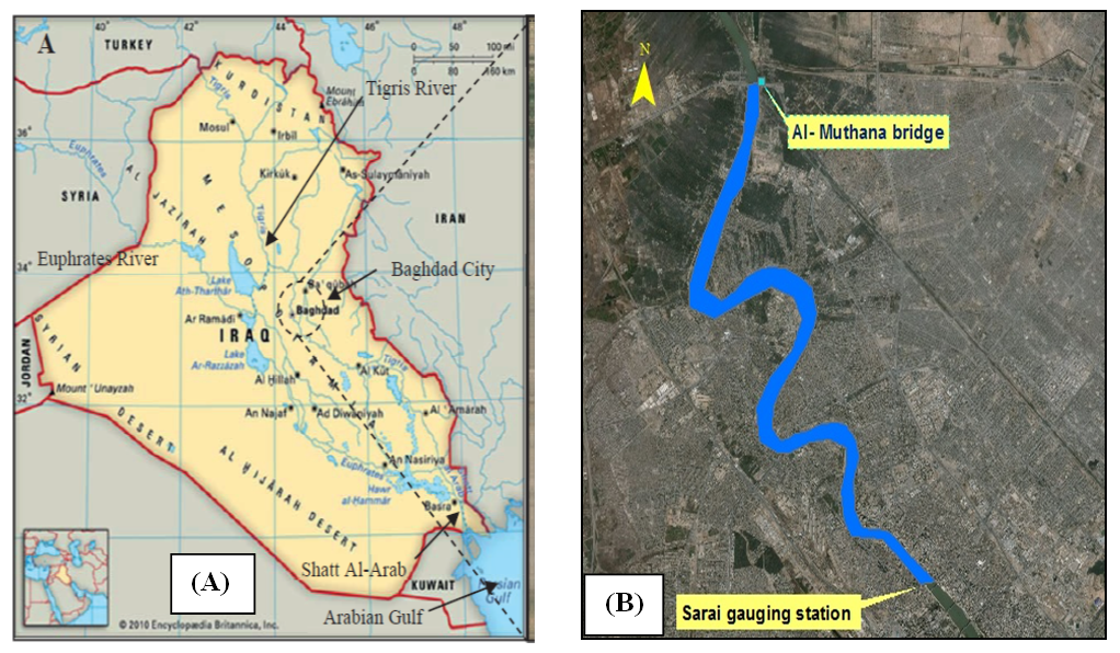 | Figure 1. (A) Map of Iraq (B) The Tigris River between Al- Muthana Bridge and Sarai gauging station at Baghdad city |
3. Theoretical Basis
3.1. One Dimensional Steady Flow
Water surface profiles are computed from one cross section to the next by solving the Energy equation with an iterative procedure called the standard step method. The Energy equation is written as follows: | (1) |
Where:  = elevation of the main channel inverts,
  = depth of water at crosss sections
  =average velocities (total discharge / total flow area),
  = velocity weighting coefficients,
  = gravitational acceleration,
  energy head loss. The energy head loss,
  between two cross sections is comprised of friction losses and contraction or expansion losses. The equation for the energy head loss as follows:
 | (2) |
Where: L = discharge weighted reach length,  representative friction slope between two sections C = expansion or contraction loss coefficient, [5].
3.2. Sediment Transport Capacity
Because different sediment transport functions were developed under different conditions, a wide range of results can be expected from one function to the other. Therefore, it is important to verify the accuracy of sediment prediction to an appreciable amount of measured data from either the study stream or a stream with similar characteristics. It is very important to understand the processes used in the development of the functions in order to be confident of its applicability to a given stream. Typically, sediment transport functions predict rates of sediment transport from a given set of steady-state hydraulic parameters and sediment properties. Some functions compute bed-load transport, and some compute bed-material load, which is the total load minus the wash load (total transport of particles found in the bed). In sand-bed streams with high transport rates, it is common for the suspended load to be orders of magnitude higher than that found in gravel- bed or cobbled streams. It is therefore important to use a transport predictor that includes suspended sediment for such a case. The following sediment transport functions are available: Ackers-White, Engelund-Hansen, Laursen, Meyer-Peter Muller, Toffaleti and Yang. The researcher must select the suitable method that the model software will deal with equations of formula, [5]. In this study the adopted formula that adopted is “Laursen”. (Laursen, 1958) derived the total sediment load predictor from a combination of qualitative analysis, original experiments, and supplementary data. Transport of sediments is primarily defined based on the hydraulic characteristics of mean channel velocity, depth of flow, energy gradient, and on the sediment characteristics of gradation and fall velocity. Contributions by (Copeland, 1989) extend the range of applicability to gravel-sized sediments. The range of applicability is 0.011 to 29 mm, median particle diameter. The general transport equation for the Laursen (Copeland) function for a single grain size is represented by: | (3) |
 Sediment discharge concentration, in weight/volume,
  Unit weight of water,
  Mean particle diameter, D = Effective depth of flow,
  Bed shear stress due to grain resistance,
  Critical bed shear stress.
  Particle fall velocity and
  Shear velocity.
3.3. Evaluation of HEC-RAS Model Performance
Three statistical criteria were used to assess the performance of the HEC-RAS model ie1- Coefficient of determination (R2): describes the proportion of the variance in measured data explained by the model. R2 ranges from 0 to 1, with higher values indicating less error variance, and typically values greater than 0.5 are considered acceptable [15].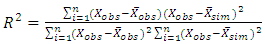 | (4) |
2- Nash-Sutcliffe efficiency (NSE): The Nash-Sutcliffe efficiency (NSE) is a normalized statistic that determines the relative magnitude of the residual variance compared to the measured data variance [13]. NSE indicates how well the plot of observed versus simulated data fits the 1:1 line. NSE is computed as shown in equation (5): | (5) |
NSE ranges between −∞ and 1.0 (1 inclusive), with NSE = 1 being the optimal value. Values between 0.0 and 1.0 are generally viewed as acceptable levels of performance, whereas values <0.0 indicates that the mean observed value is a better predictor than the simulated value, which indicates unacceptable performance.3- RMSE-observations standard deviation ratio (RSR): RMSE is one of the commonly used error index statistics [6]. Although it is commonly accepted that the lower the RMSE the better the model performance, only [5] have published a guideline to qualify what is considered a low RMSE based on the observations standard deviation. Based on the recommendation by [16] a model evaluation statistic, named the RMSE-observations standard deviation ratio (RSR), was developed. RSR standardizes RMSE using the observations standard deviation, and it combines both an error index and the additional information recommended by [9]. RSR is calculated as the ratio of the RMSE and standard deviation of measured data, as shown in equation (6): | (6) |
Where the observed value variable.
 the simulated value variable.
 Mean of the simulated values variable.
4. Methodology and Data Requirement
4.1. One Dimensional Steady Flow
Either geometric data can be entered directly in HEC-RAS from the geometric data editor, or it can be developed in Arc GIS, using HEC-Geo RAS, and then imported into the HEC-RAS Geometric data editor. The newest cross-sections can be invested in this study for the stream bed surface to be a part of available 78 cross-sections which requires. Upstream of a reach, it is assumed that the flow remains constant until another flow value is encountered within the reach. By using the records of flow rate, which obtained from the [11], for (87years), Figure 2, which represents the flow rate in Tigris River at Sarai gauging station for the period (1930-2017). Four scenario of the flow value (minimum, average, maximum and flood) can be established to simulate the flood plane for Tigris River. The next step is to select the desired flow regime for which the model will perform calculations. Subcritical flow is the selected flow regime. The selected flow rates were 461, 890, 1815 and 2500 m3/sec with return period time (1, 2,87 and 300 year), were survived along the Tigris River between Al- Muthana bridge and Sarai gauging station. The study reach starts at upstream side (section 1) at Al- Muthana bridge to (section 78) at Sarai gauging station which represents the downstream of the river reach. The geometric data conducted by [11]. Cross sections to be ordered within a reach from the highest river station upstream to the lowest river station downstream. The reach is defined by (78) cross sections distribution every (250 m), numbered from (19500) to (250 as shown in the Figures 3 and 4. In this study, just four bridge data are introduced (Al-A'amah bridge, Al -Adamiyah bridge, Al- Sarafia bridge and Bab Al-Muadam bridge). All data concerning with designing of bridge in upstream and downstream of bridge station represent an input data, these are: place of bridge, inter outer border of bridge (Deck/Roadway) data, slope of abutment, dimensions and elevations of piers to model the bridge approach by model. Flow data are entered from upstream to downstream for each reach. | Figure 2. Yearly flow rate for Tigris River at Sarai gauging station for the period (1930-2017) |
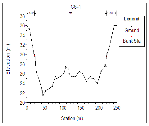 | Figure 3. Cross section (CS-1) |
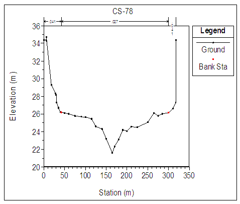 | Figure 4. Cross section (CS-78) |
4.2. Morphological Model (1-D Mobile Bed Sediment Routing Model)
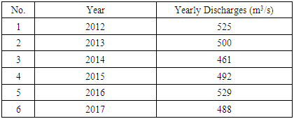
The quasi-unsteady approach approximates a flow hydrograph by a series of steady flow profiles associated with corresponding flow durations. HEC-RAS includes several quasi-unsteady boundary conditions, but only one upstream quasi-unsteady boundary type. Each upstream boundary (the upstream cross section of an open-ended upstream reach) requires a flow series boundary. HEC-RAS includes three options for setting quasi-unsteady downstream boundary conditions: Stage Time Series, Rating Curve, or Normal Depth. HEC-RAS requires external (upstream and downstream) boundary conditions to run sediment analyses. The Quasi-Unsteady flow editor automatically used an external boundary cross sections, and required boundary conditions. For an upstream external boundary, flow Series must be chosen, which was based on a Computational Increment in (hours); Flow Duration in (hours); and Flow in (m3/s). Each downstream boundary can be Stage Time Series, Rating Curve, or Normal Depth. In this study, a "Normal Depth" was selected for downstream boundary condition. Table 1 shows the average yearly flow rate, which is used in Morphological Model. Each cross section requires initial bed gradation data. According to the [8] that presented a study for reach of Tigris river Baghdad, which contained a sieve analysis for samples from bed of the river. To assign bed gradations to the cross section, first create bed gradation templates. The bed gradation represents the grain size distribution of the particles. Figure 5: A and B show the grain size distribution of the particles illustrated by a logarithmic diagram for the upstream and downstream of the Tigris river reach, respectively. Present Finer defines the sample using as a cumulative bed gradation curve with percent finer defined by the upper bound of each grain class. The diameter listed for each grain class is the upper bound of that grain class and values should be entered as percents.Table 1. The average yearly flow rate, which is used in Morphological Model
 |
| |
|
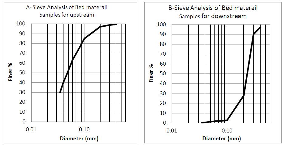 | Figure 5. The grain size Distribution (Geohydraulique, 1980) |
4.3. Sediment Transport Capacity Model
The sediment transport capacity function in HEC-RAS has the capability of predicting transport capacity for non-cohesive sediment at one or more cross sections based on existing hydraulic parameters and known bed sediment properties. It does not take into account sediment inflow, erosion, or deposition in the computations. Classically, the sediment transport capacity is comprised of both bed load and suspended load, both of which can be accounted for in the various sediment transport predictors available in HEC-RAS. Results can be used to develop sediment discharge rating curves. Sediment Transport Capacity model in this study depends on Bathymetric Surveys that conducted by [11]. The same cross-sections used for flood routing model and the same calculated values for the hydraulic sections will be used within the HEC-RAS program to estimate for the calculation of sediment transport capacity model. Figure 6: A shows the rating curve for the total sediment which calculated by, [8]. The flow rates are ranging between 500 to 3500 (m3/s). Figure 6: B shows the rating curve for the total sediment by [3], which prepared from all data regression (all historical records), and used the same range of flow rate that used in Figure 6: A. [8], will be used in the calibration of the sediment transport model, and the rating curve for total sediment by, [3] will be used in the verification process of the sediment transport capacity. The difference of the total load sediment between the [8] study and [3] study belongs to many points. (1) Selection the formulas that calculates the total sediment (2) the methods of sampling (3) the number of samples (4) concentration of sediment and another reasons such as the varying of the river geometry and training of the river. [1], collected forty six sediment samples from the bed of Tigris River within Baghdad City at 15 cross section and the cumulative curves (% Finer) were drawn according to the obtained results of laboratory test and analysis, Figure 7.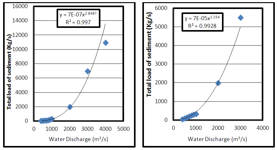 | Figure 6. (A) Rating curve for total sediment by [8] (B) Rating curve for total sediment by [3] |
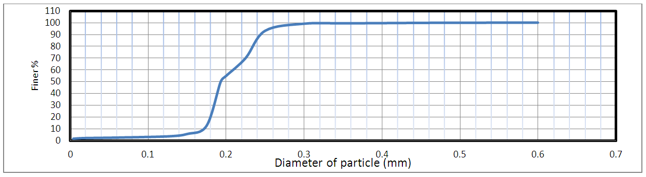 | Figure 7. Cumulative curve of the bed sediment (percentage Finer) of Tigris River at Baghdad [1] |
5. Results and Discussion
5.1. Calibration of HEC-RAS Model for n Manning Roughness Coefficient
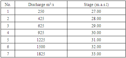
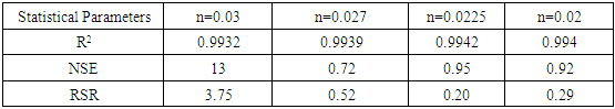
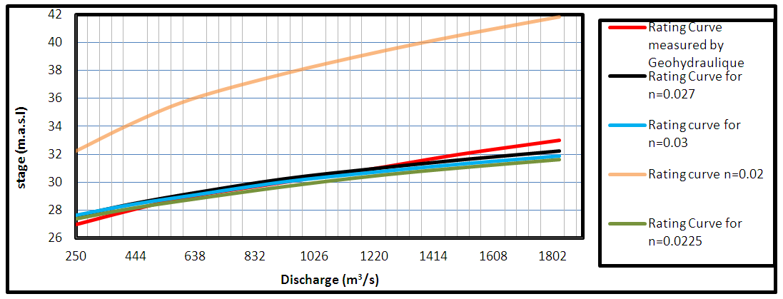
The Calibration process was achieved by using the recorded data during the period from 1976 to 1980 at Sarai station, Table 2 shows the measured water surface elevation relative to flow rate conducted by [8] which was used in the Calibration process for a range of river discharges started from 250 to 1815m3/s, with increment interval of 200 m3/s. A comparison between the measured by [8] and model predicted rating curves showed that the roughness coefficient is equal to (0.02, 0.0225, 0.027 and 0.03) for the main channel and 0.038 to 0.042 for the left and right banks Figure 8. Obviously, Figure 8 shows that the value (0.027) closest to the measured rating curve of the Tigris River. Table 3 shows the values of (R2), NSE and RSR. The roughness coefficient was equal to (0.027) for the main channel and 0.041 for the left and right banks which record a good accuracy, therefore these values can be used in the HEC-RAS model.Table 2. The measured stage relative to flow rate conducted by [8]
 |
| |
|
Table 3. The values of (R2), NSE, and RSR for The roughness coefficient
 |
| |
|
 | Figure 8. Calibration process for n values by HEC-RAS model |
5.2. One Dimensional Steady Flow
As an underlying perspective of the steady flow analysis output, from the principle program window view and after that water surface profiles were chosen. This enacted the water surface profile as appeared in (Figure 9) from this profile. This figure was generated by running the model with discharges 461, 890, 1815 and 2500 m3/sec, which repre sents minimum, average, maximum and flood flow discharge respectively. It is clearly from (Figure 9) that there is no inundation along the reach because the reach protected by high banks and lined by rocks from the left and right, but if the discharge is higher than maximum flow which is equal to 2500 m3/sec a critical state appears in some stations especially the station from (11250) to (12250) along the reach. However, the four water surface elevation (minimum, average, maximum and flooding) at the upstream is equal to (28.96, 30.24, 32.36 and 33.45) (m.a.s.l) and for downstream of the reach (26.67, 27.62, 29.14 and 30.06) (m.a.s.l), respectively. Figure 10 shows the velocity at Sarai gauging station is equal to 1.72 m/s for flooding discharge (2500 m3/sec), this value is acceptable with The measurements of the velocity that were conducted by [8] at the Sarai gauging station which was ranging between 1.2 to 2.4 m/s for flow rate (2500) m3/sec. A rating curve is a relationship between stage and discharge at a cross section of a river. The outlet-rating curves were illustrated in Figure 11. One of the disadvantage for HEC-RAS Model, that the equation of the rating curve is not given in the output of the Model so the output values from the model of the stages m and discharge in m3/sec were drawn in Figure 11. The best fit of these values were a power equation. The curve are generally expressed in the form of a power-law type equation for the rating curve of the Figure 11, (Eq. 7) was established with a coefficient of determination (R2) of (0.95): 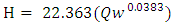 | (7) |
Where H: Water Surface Elevation in (m) Water discharge in (m3/s)
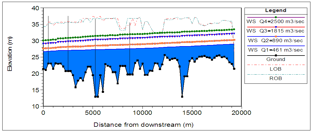 | Figure 9. Four water surface profiles by HEC-RAS model |
 | Figure 10. Longitudinal average velocities along the river reach for four values of discharge (461, 890, 1815 and 2500 m3/sec) |
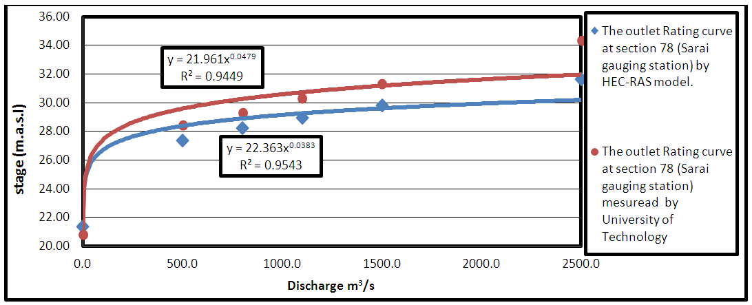 | Figure 11. The outlet Rating curve at section 78 (Sarai gauging station) |
Moreover, Figure 11 can be used to compare the predicted results of rating curve with measured rating curve by [17] for downstream by using the two statistical criteria (NSE, RSR) to assess the performance of the (Eq. 7), The value of (NSE) was equal to (0.9917). Additionally the (RSR) was equal to 0.14.
5.3. Morphological Model (1-D Mobile Bed Sediment Routing Model)
The invert of a river is an important criterion in geometry of the river cross section to define the potential of erosion or deposition. It undergoes changes during the time affected from river phenomena. The HEC-RAS model has the capability of drawing the spatial plot for many hydraulic characteristic like velocity. Water surface elevation, shear stress and geometric characteristic like invert change of bed for all cross section. For this purpose, Figure 12 shows the longitudinal invert of the reach at the start and the end of the period from 2/10/2012 to 2/10/2017 relative to the average yearly flow rate as shown in Table 2, The invert change in the model was produced using Ackers White sediment transport function, the difference between invert change in each cross section and initial bed level will determine the sedimentation. If the invert change is lesser than the initial bed level, then deposition takes place in that particular cross section and vice versa. Figure 13 shows the invert change with respect to the initial invert of the river bed at the various cross sections in the study reach from during the period between 2012 to 2017 year. The maximum cumulative depth of erosion in the reach is about 2.07 m occurring at River Station 500 (from upstream) and the maximum cumulative depth of deposition is about 1.45 m at River Station 5500 (from upstream) of river as shown in Figure 13, in which the negative and positive value refers to the erosion and deposition processes, respectively. The erosion is located in the upstream and downstream of the reach, and the deposition is concentrated in the middle of the river reach, especially at the meandering. The average depth of erosion and deposition are equal (0.51 and 0.39 m), respectively. Figure 14 shows the initial bed elevation and the predicted bed elevation in the year 2040 for the flow cases of 461 m3/s. In this model the maximum discharge was not used because the program records error with note "unrealistic results" therefore it has been the excluded of the maximum discharge, respectively. It is clearly, the degradation is the general case for the bed elevation of Tigris river reach which it will occur by erosion processes, and the degradation increased relatively with the increase in flow rate as shown in Figures (12,13,14), especially in the beginning of the reach of the study from station (0) to station (4500m) because no meandering in this region. The reasons of why these cross sections subjected to high erosion as previously presented. The average depth of degradation in the bed elevation of Tigris river reach within Baghdad city between the years 2012 and 2040 was approximately equal to 1m for flow rate 461 m3/s.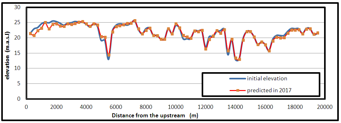 | Figure 12. The longitudinal profile of the bed invert elevation change during the period from 2/10/2012 to 2/10/2017 |
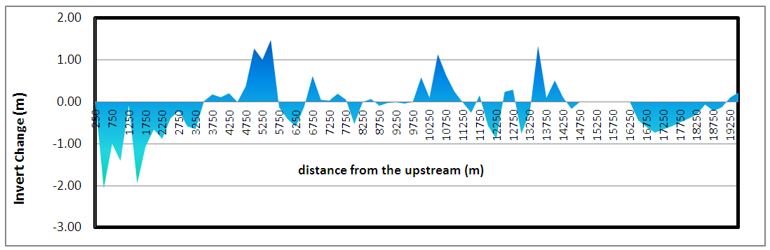 | Figure 13. The cumulative invert change with respect to the initial invert river bed in 2017 |
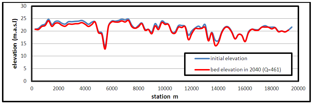 | Figure 14. The initial bed elevation and the predicted bed elevation in 2040 for Q=461 m3/s |
5.4. Sediment Transport Capacity Model
In general, the sediment discharge increases with an increase in river discharge, so, sediment-rating curve is a good empirical method to investment the total load of sediment. A sediment-rating curve is a relation between the sediment load and river discharges. Such a relationship is usually established by regression analysis, and the curves are generally expressed in the form of a power-law type equation. For the study reach, the power equation for the data of total sediment load with respect to flow discharge that predicted by HEC-RAS model Laursen (Copeland) equation, is shown in (Eq. 8) and Figure 15 with determination coefficient (R2) of (0.981). The sediment rating curve is as follow: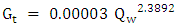 | (8) |
Where  total sediment discharge (kg/s).
 Water discharge (m3/s).
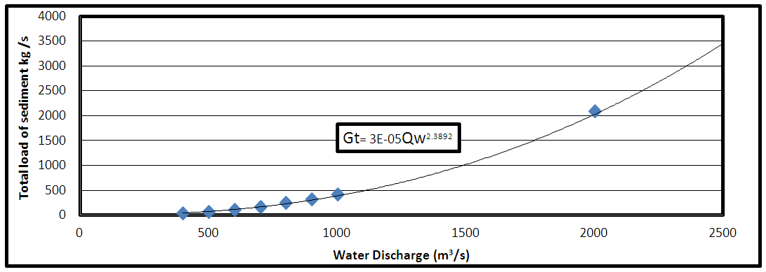 | Figure 15. The total load-rating curve along the northern reach of the Tigris River in Baghdad city that predicted by HEC-RAS model |
5.5. The Verification of Rating Curve Sediment Transport Capacity
The verfication can be make for the rating curve of sediment transport capacity model. Figure 16: shows the comparison between measured results by [3] with respect to the Computed Results of the rating curve of sediment transport capacity model by Laursen (Copeland) in the HEC-RAS model for this study. Figure 17 shows the correlation between the measured total load of sediment and the values calculated by Laursen equation. The value of coefficient of determination (R2) was equal to (0.9917). Additionally the NSE and RSR were equal to 0.969 and 0.173, respectively.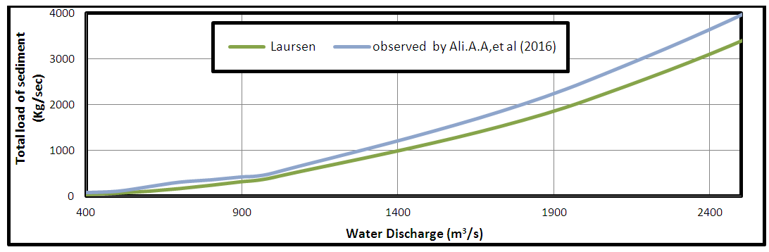 | Figure 16. Comparison between the rating curve of the sediment transport capacity at Sarai gauging station and measured results by [3] |
 | Figure17 . Correlation between observed and computed results of the rating curve for the total load sediment |
6. Conclusions
This study introduces the application of the HEC-RAS (Simulation of the water flow, morphological changes, sediment transport capacity) model. The main targets are to develop and examine the ability of the model. Corresponding to the results of the 1-D Steady flow model obtained by this study, the following conclusions may be shown as: 1- This study presented the new formula for estimating the water level surface corresponding to the flow rate of the rating curve for the downstream of the Tigris river reach within Baghdad. The flow regime reach was subcritical with average Froude number of (0.17). The average energy slope was 10 cm/km. The velocity at Sarai gauging station is equal to 1.72 m/s for the flooding discharge (2500 m3/sec). This value is acceptable with the measurements of the velocity that were measured by [8], at the Sarai gauging station which was ranging between 1.2 to 2.4 m/s for flow rate (2500) m3/sec.2- For the calibration of the HEC-RAS model, the optimum value of the manning coefficient was 0.027 for main channel and 0.041 for banks.3- the elevation of water surface is ranging between 26.67 and 33.45 (m.a.s.l) for all the scenarios of flow rate values.The results of analysis of morphological model (Mobile Bed Sediment Routing Model) of the Tigris River led to following conclusions: 1- The erosion is located in the upstream and downstream of the reach, and the deposition is concentrated in the middle of the river reach, especially at the meandering. The average depth of erosion and deposition are equal to (0.51 and 0.39 m), respectively.The results of analysis of the sediment transport capacity of the Tigris River led to following conclusions: 1- Laursen (Copeland) formula showed a good agreement with the measured data. 2- This study presented a new formula for estimating the total load sediment corresponding to the flow rate of the rating curve for the downstream of the reach Tigris river within Baghdad city. 3- The HEC-RAS model, shows an excellent suitability in simulation scattering values of change of sediment transport capacity which were compared with the measured values.
References
| [1] | Al-Ansari, Nadhir, Ammar A. Ali, Qusay Al-Suhail, and Sven Knutsson. (2015) 'Flow of River Tigris and Its Effect on the Bed Sediment within Baghdad, Iraq', Open Engineering Vol.5, pp.465–477. |
| [2] | Ali A. A., Al-Ansari N. A., and Knutsson S. (2012), 'Morphology of Tigris River within Baghdad City', Journal of Hydrology and Earth System Sciences, Vol. 16, pp. 3783–3790. |
| [3] | Ali A. A. (2016) "Three Dimensional Hydro- Morphological of Tigris River". A thesis submitted to Lulea University of Technology. Sweden. |
| [4] | Brunner. Gary. W. (2016), HEC-RAS River Analysis System User ' S Manual, US Army Corps of Engineers Hydrologic Engineering Center. |
| [5] | Brunner, Gary W. 2016. “HEC-RAS River Analysis System.” Hydraulic Reference Manual Version 5.0. US Army Corps of Engineers Hydrologic Engineering Center. |
| [6] | Chu, T. W., and A. Shirmohammadi. 2004. Evaluation of the SWAT model’s hydrology component in the piedmont physiographic region of Maryland. Trans. ASAE 47(4): 1057-1073. |
| [7] | D. N. Moriasi, J. G. Arnold, M. W. Van Liew, R. L. Bingner, R. D. Harmel, T. L. Veith. 'Model Evaluation Guidinless For Systematics Quantivication of Accuraccy cultural and Biological Engineers ISSN 0001−2351. |
| [8] | Geohydraulique, 'Tigris River Training Project within Baghdad City', Unpublished Report Submitted to the Iraqi Ministry of Irrigation, Paris, 1980. |
| [9] | Legates, D. R., and G. J. McCabe. 1999. Evaluating the use of “goodness-of-fit” measures in hydrologic and hydroclimatic model validation. Water Resources Res. 35(1): 233-241. |
| [10] | Ministry of Water Resources, "bathometric survey, (2012)", unpublished data. |
| [11] | National Center of Water Resources Management, "flow data, (2017)", unpublished data. |
| [12] | Nama A. H., (2015), 'Distribution Of Shear Stress In The Meanders Of Tigris River Within Baghdad City', Al-Nahrain University, College of Engineering Journal (NUCEJ) Vol.18 No.1, pp.26-40. |
| [13] | Nash, J. E., and J. V. Sutcliffe. 1970. River flow forecasting through conceptual models: Part 1. A discussion of principles. J. Hydrology 10(3): 282-290. |
| [14] | Sh, Thair, and Ayad S Mustafa. (2013). 'Multiple Linear Regression Model for Suspended Load Transport Rate Prediction and Its Evaluation Using Selected Transport Formulas.' International Journal of Civil & Environmental Engineering IJCEE-IJENS Vol:13 No:06. |
| [15] | Santhi, C, J. G. Arnold, J. R. Williams, W. A. Dugas, R. Srinivasan, and L. M. Hauck. 2001. Validation of the SWAT model on a large river basin with point and nonpoint sources. J. American Water Resources Assoc. 37(5): 1169-1188. |
| [16] | Singh, J., H. V. Knapp, and M. Demissie. 2004. Hydrologic modeling of the Iroquois River watershed using HSPF and SWAT. ISWS CR 2004-08. Champaign, Ill.: Illinois State Water Survey. Available at: www.sws.uiuc.edu/pubdoc/CR/ISWSCR2004-08.pdf. Accessed 8 September 2005. |
| [17] | University of Technology, 'Training of Tigris River inside Baghdad City', unpublished report submitted to the Iraqi Ministry of Agriculture and Irrigation, Baghdad, 1992. |

 Abstract
 Reference
 Full-Text PDF
 Full-text HTML