F. Boushaba, A. Yachouti, S. Daoudi, I. Elmahi
Civil Engineering, University of Mohamed first, ENSA (National School of Applied Sciences) Oujda, Morocco
Correspondence to: F. Boushaba, Civil Engineering, University of Mohamed first, ENSA (National School of Applied Sciences) Oujda, Morocco.
| Email: |  |
Copyright © 2017 Scientific & Academic Publishing. All Rights Reserved.
This work is licensed under the Creative Commons Attribution International License (CC BY).
http://creativecommons.org/licenses/by/4.0/

Abstract
This paper is divided into two parts: The first part is the modeling of the kinetic energy dissipation provided by the flood wave in the presence of different geometric shape roughness along the canal. We use a new version of Roe scheme named SRNH written in finite volumes method. This is to model the spread of a flood wave along the canal equipped with regularly spaced identical grooves which plays the role of macro roughness. Water flow is simulated on three different geometrical shapes; a smooth rectangular channel, channel with roughness as rectangular and trapezoidal grooves, note that wet surfaces are the same for all three configurations. The purpose of this simulation is looking for the form that realizes the maximum kinetic energy dissipation provided by the flood wave. The second part consists of modeling the influence of sediment transport in the presence of macro roughness, it is assumed that the bed of the channel moves with the free surface of the water. The bed is composed of fine sand size. For sediment transport we use Meyer-Peter-Muller model. Finally we observe the influence of macro roughness on the transport and deposition of sediments.
Keywords:
Finite volumes, Saint-Venant equations, Macro roughness, Sediment transport
Cite this paper: F. Boushaba, A. Yachouti, S. Daoudi, I. Elmahi, Finite Volume Scheme Simulation of Unsteady Flow in Channel with Different Macro Roughness: Application to Regular and Non Regular Canal with Sediment Transport, International Journal of Hydraulic Engineering, Vol. 6 No. 1, 2017, pp. 9-15. doi: 10.5923/j.ijhe.20170601.02.
1. Introduction
Surrounding Dissipation techniques have been used in various fields, among which there is the application of this technique in dam break, the impact of jets of weirs, the spillways that are present in many industrial hydraulic applications. In the case of large dams, spillways flood jets have very high speeds, especially during flood where drainage systems often operate at full capacity. The given kinetic energy has to be dissipated to prevent damage of hydraulic structures. A typical solution is the dissipation energy of the flood wave by the direct impact of roughness created on canal banks.Knowledge of the flow characteristics is fundamental to assess the stability of the structure or understand and simulate the protective structure development process. This analysis will help to avoid risks for projects located downstream of the water flow. In addition to the design of hydraulic structures we should take into account erosion bed phenomena in rivers. Such problems require knowledge of basic principles, especially the calculation of velocity fields and its influence against macro roughness placed along the canal and erosion of the bottom. Several engineering techniques are used to increase the lifespan of the hydraulic structures, that include threshold stairs, single and double containment basins, macros roughness etc. In the first part of the paper, we study three different channel configurations, smooth rectangular channel, rectangular channel with five rectangular macro roughness arranged on different locations on the two banks and rectangular channel with five trapezoidal macro roughnesses. With the same sinusoidal flood wave through the three configurations, we compare the dissipation of kinetic energy created by the flood wave crossing the rough macros. In the second part, we conclude with the simulation variable background due to the erosion of the channel bed.
2. Mathematical Formulation Model and Governing Equations
The model usually used to describe the free surface flows is based on the two-dimensional Saint-Venant equations. These quite known models in the literature equations, are obtained by integrating the vertical dimensional incompressible Navier-Stokes equations under the assumptions of hydrostatic pressure and averaged velocities in the vertical level. Terms from the turbulence, viscosity, and the Coriolis forces are not considered in this study. The system can be set as conservative form: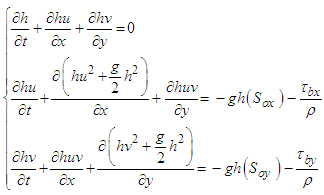 | (1) |
where u and v are the depth-averaged water velocities in x and y direction, h the water depth, g the gravitational acceleration,  and
and  are respectively slopes following the direction x and y. They are defined by
  and
and  z is the bottom topography, τbx and τby the bed shear stress in the x and y direction, respectively, defined by the depth-averaged velocities as:
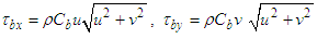 | (2) |
where Cb is the bed friction coefficient, which may be either constant or estimated as  , where
  is the Chezy constant, with nb being the Manning roughness coefficient at the bed. To update the bedload, we consider the Exner equation given by
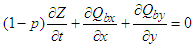 | (3) |
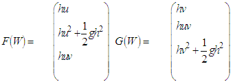
where p is the sediment porosity assumed to be constant, Qbx and Qby represent the bedload sediment transport fluxes in x- and y-direction, respectively. These fluxes depend on the type of sediment and for simplicity in the presentation, we consider the basic sediment transport fluxes [6]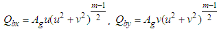 | (4) |
with m and Ag are coefficients usually obtained from experiments taking into account the grain diameter and the kinematic viscosity of the sediment. In practice, the values of the coefficient Ag are between 0 and 1 depending on the interaction between the sediment transport and the water flow. We can write the system of equations (1) as conservative form: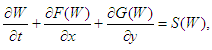 | (5) |
where W is conservative variables vector, F and G are the advective flow functions and S is the source term.
3. Solution Procedure for Bedload Equation
The bedload formulate by equation (3) involves different physical mechanisms occurring within different time scales according to their time response to the hydrodynamics. In practice, the sediment transport of the bed occurs on a transport time scale much longer than the flow time scale, compare for example [2-4]. In the present work, we have adopted the quasi-steady approach studied in [3]. This approach consists of separately solving the shallow water equations (5) to an equilibrium state keeping the fixed bed followed by a sediment transport step where the bed is updated in (3) keeping the velocity field and fixed water height. Hence, to numerically solve equations (5) and (3), we apply a method early developed in [2, 3] for solving sediment transport equations using the bed discharge function (4). The method was also investigated by the authors in [1] for shallow water flows on fixed beds. Our focus in the current study is to check the performance of the method to for solve morphodynamic models in contracting channel flows. Therefore, we briefly describe the numerical method and we refer the reader to [1-3] for more details.The numerical solution of the equation system (5) has a lot of numerical difficulty and is still subject of much recent work. Indeed, the non-linear nature of this combined with its hyperbolicity excludes the use of analytical techniques for most practical problems, in addition, it can lead to discontinuous solutions (hydraulic jumps) even if the initial data is regular. On the other hand, the presence of the terms of steep slopes forms the irregularity of the bottom, and makes the most existing conventional schemes inappropriate.In this paper we use the Non Homogeneous Riemann Solver (SRNH).
4. Finite Volume Discretization Equation
The finite volume formulation begins with the discretization of the computational domain with a finite volume control. Finite volume formulation is considered here "cell-centered" which assumes that the volume controls coincide with the triangles of the mesh and the unknowns variables are the mean states on each volume controls (see illustration below).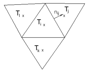 | Figure 1. Cell-centered |
By integrating the system (5) on a volume control  and using the Green's divergence formula, the following complete system is obtained:
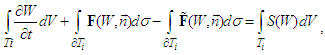 | (6) |
where the convective flow and distribution functions are defined by: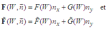
 is the triangle border of
  and
and  the outer unit normal to
4.1. SRNH Scheme
We use a numerical method of finite volume, based on a Non Homogeneous Riemann Solver (SRNH) recently developed in [1, 8] for non-homogeneous hyperbolic systems. The construction of the numerical scheme is based on the hyperbolicity of the system and the self-similarity of the solution. The SRNH scheme is formulated by considering only the hyperbolic part of the system (5) and the source term describing the background of the domain: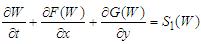 | (7) |
The algorithm has two stages: a predictor and corrector stage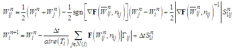 | (8) |
 is the length of the edge
  separates triangles
  and
and 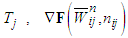 denotes the Jacobian of F calculated at the average state
  of Roe at time
 represents the sign matrix of
  This matrix is determined by the projection of the Saint-Venant equations on the normal interfaces, it can reduce the components of the source term and write predictor step in one direction [1].One feature of this solver is the ability to check the exact conservation property (also known as C-property) and ensures the positivity of the water level for unsteady flows.
4.2. Second Order Extension
Note that the discretization (8) is only first-order accurate. In order to develop a second-order finite volume method, we use a MUSCL incorporating slope limiters in the spatial approximation and a two step Runge–Kutta method for time integration. The MUSCL discretization uses an approximation of the solution state W by linear interpolation at each cell interface  as
as | (9) |
where  and
and  are the barycenter coordinates of cells Ti and Tj, respectively. Thus, the cell gradients are evaluated by minimizing the quadratic functional
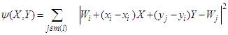 | (10) |
where m(i) is the set of indices of neighboring cells that have a common edge or vertex with the control volume Ti. To obtain a TVD scheme, the VanAlbada slope limiter is incorporated to the reconstruction (9)–(10), see for instance [5].The resulting scheme preserves the positivity of the water depth and it is a well balanced scheme, which is very important in the case of free surface flows on variables bed. A test on the equilibrium property of the SRNH scheme is performed in reference [1].
5. Numerical Results
To verify the influence of macro roughness on the dissipation of kinetic energy through the channels, we solve the transportation of a sine flood wave along three channels with different geometric shapes; smooth rectangular channel, rectangular channel with rectangular macro roughness and rectangular channel with trapezoidal macro roughness In Fig.2 we display the geometry of each configuration.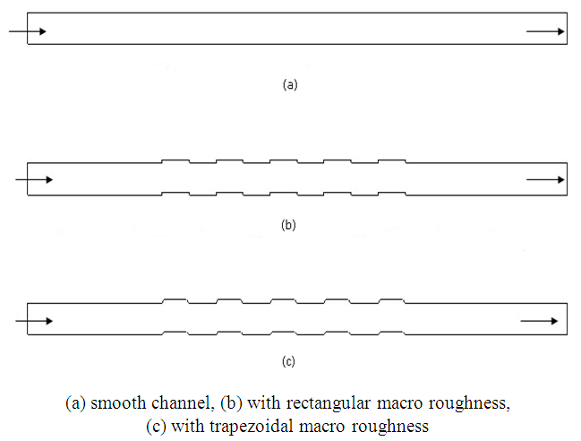 | Figure 2. Domain for the channel model |
In Fig. 3 we display the fine fixed triangular meshes.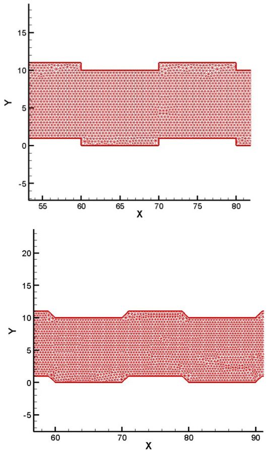 | Figure 3 |
The boundary conditions are Neumann type for speed and height. For the rest of the domain, sinusoidal flood wave is imposed: The initial conditions are:
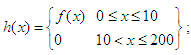
5.1. Results for the Rectangular Channel with Rectangular Macro Roughness
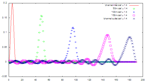
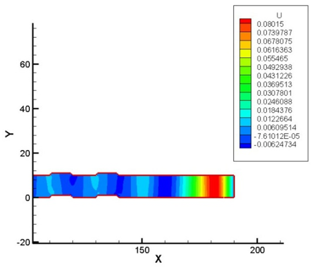
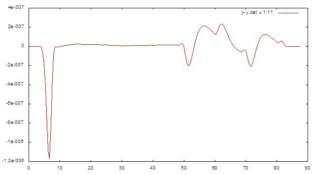
Firstly we consider the channel with rectangular macro roughness with zero slope and a rigid bottom. Fig. 5.1-a shows the flood wave velocity field captured at the entrance of the channel before the macro roughness. After the travelling of the sine wave along the channel, we see a consistent dissipation of the velocity amplitude. Indeed some of the dissipation speed is due to the diffusive nature of finite volume scheme, however the presence of obstacles along the canal also contribute to the reduction of the kinetic energy provided by the wave created by the speed weakening see fig 5.1-b.Continues line: Initial configuration of the wave, diamond dotted line: wave at 50m, + dotted line: wave at 100m, rectangular dotted line: wave at 150m, X dotted line: wave at the output of the channel.Figure 5.1 c shows a section through the longitudinal axis of the channel, with the amplitude of the sine wave velocity. The solid line of the graph represents the amplitude of the velocity at the entrance of the channel, while the last of the outline symbol x represents the amplitude of the velocity at the outlet of the channel. It can be observed that the speed has dissipated, especially through the barriers on both sides constituting from the macro roughness. We also, we observes a series of secondary reflected waves, because of singularities (shock at the both sides of the channel). We can conclude that macro roughness could stifle the kinetic energy provided by the wave flood. | Figure 5.1-a |
 | Figure 5.1-b |
 | Figure 5.1-c |
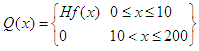
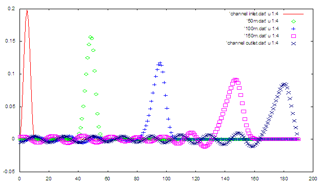
5.2. Results for the Rectangular Channel with Trapezoidal Macro Roughness
We carry the same simulation scenario as the rectangular roughness model. We assume that the trapeze and rectangular macro roughness have the same value of the wet surface.Figure 5.2 a and Figure 5.2 b show the evolution of the velocity along the channel, Figure 5.2-c shows the dissipation rate of the flood wave along the canal. We note the presence of a series reflected waves downstream of the channel because of the roughness placed along the canal.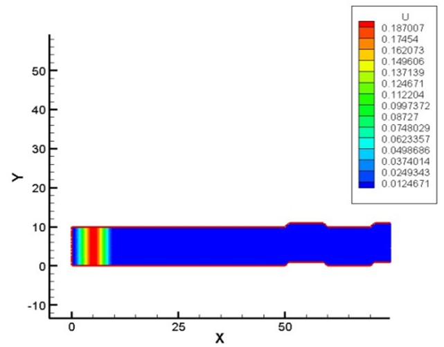 | Figure 5.2-a |
 | Figure 5.2-b |
 | Figure 5.2-c |
Continues line: Initial configuration of the wave, diamond dotted line: wave at 50m, + dotted line: wave at 100m, rectangular dotted line: wave at 150m, X dotted line: wave at the output of the channel.
5.3. Comparison of Three Configurations
We compare the evolution of the sine wave through the three forms of channels.Figure 5.3 a shows a comparison of the dissipation of the kinetic energy at the entrance and exit of the channel for the three test cases (rectangular channel with macro rectangular and trapezoidal roughness and smooth channel). There is a slight difference between dissipation trapezoidal and rectangular, We confirm with the numerical simulation of the velocity field that the channels with the five macro roughness dissipates the kinetic energy with a rate of 10% more than the smooth channel.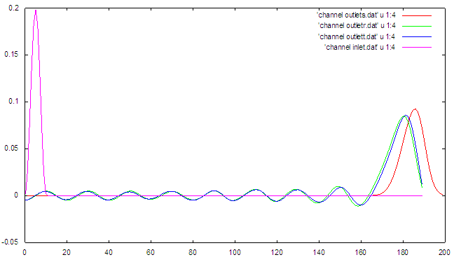 | Figure 5.3-a |
Legend (Channel outlets: smooth channel, Channel outlet: channel with rectangular roughness, Channel outlet: channel with trapezoidal roughness, Channel inlet: initial wave.)For clarity, we zoom the basis of wave, see Figure 5.3b. The incident wave is decomposed after passing along the singularities in a main transmitted wave and a series of reflected wave, we note that the reflected wave in the case of rectangular channel with macro roughness is slightly larger than the channel with macro trapezoidal roughness that explains the slight difference in the rate of dissipation. This is very physical because the trapezoidal shape presents a progressive geometric change while the rectangular presents a steep geometric change.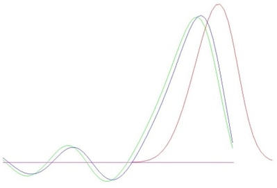 | Figure 5.3-b |
6. Flow with Sediment Transport Results
To check the proposed finite volume, we use a morphodynamic Grass model (4) in a hydraulic structure with rectangular roughness, for more details, see reference [7] which deals with represents a comparison of unstructured finite-volume morphodynamic models in contracting channel flows. Here, the parameter m= 3 and Ag = 0.001 resulting in a relatively slow interaction between the bedload and the water flow. We carry the same simulation scenario as in flow without sediment transport. Figure 6-a represents the curve of tub of the sine wave at the initial moment.For the first run, we observe that the flood wave on the surface of water in its movement causes on the bed of the canal a transport of matter (erosion) quickly followed by a deposit see figure 6-b.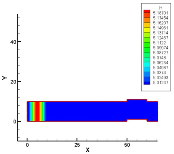 | Figure 6-a. Flood wave at the initial moment (with flat bottom) |
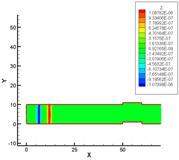 | Figure 6-b. Evolution of the bed of the channel after 2 seconds |
Now, we're going to miss the flood wave through the first macro roughness. We can see in figure 6c that the erosion and the deposition on the contraction and non-contraction zone, are well resolved in terms of location and propagation celerity. This can be explained by the variation of the kinetic energy in the vicinity of macro roughness. The area contract fact increases the speed, which crates erosion, however, in the enlarged zone the speed decreases and the material deposit phenomenon happens. 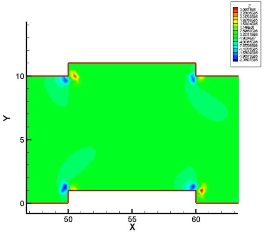 | Figure 6-c. Evolution of the canal bed during the passage of the flood wave in macros roughness |
 | Figure 6-d. Longitudinal sections at the channel vertical center y = 5m for the bed using the Meyer-Peter |
In comparing the two configurations, the transport in the smooth channel and channel with macro roughness is done in the same way at the entrance of the canal (smooth part) and the erosion is well pronounced, but once the flood wave passes through the first macro roughness we observe a phenomenon of erosion (the speed of the wave increases in the area shrunk) followed abruptly by a deposit of sediment in the extended area. However t in a smooth channel, the inertia of the wave carries the eroded sediment from the channel input and are removed slowly along the see figure 6e.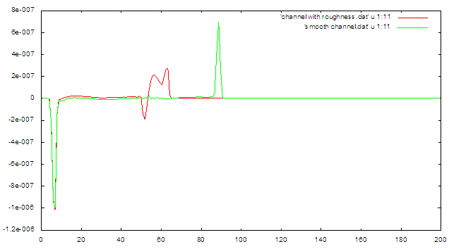 | Figure 6-e. Comparison of the transport of sediment in smooth channel and channel with macro roughness at the bed using the Meyer-Peter |
7. Conclusions
The hydraulic characteristics of the flow such as the speed and the free surface of the water (curve of tub), the transport of sediments are of the necessary data for the Design of hydraulic structures (geometry, shape). We have simulated numerically the dissipation of the kinetic energy of waves of flood. The problem was the search for the geometry of the hydraulic structure capable of dissipating the flood wave. To do so we used three types of channels, a smooth channel and a channel with rectangular roughness placed along the channel, and a third one with the trapezoidal roughness shapes. It has been confirmed that the channels with the macro roughness placed on both sides of the shore channel significantly dissipates the kinetic energy provided by the flood wave. We have studied the influence of macro roughness on the erosion and the formation of deposits along the canal, the model of Grass is used. The bed of the canal is composed of grain of sand that moves through the flow of water. The numerical results confirm that the macro roughness decrease the erosion and serves as pockets of deposit of sediment.
References
| [1] | F. Benkhaldoun, I. Elmahi and M. Seaïd. “Well-balanced finite volume schemes for pollutant transport by shallow water equations on unstructured meshes” J. Comput. Phys. (226) 180–203, 2007. |
| [2] | F. Benkhaldoun, S. Sahmim, M. Seaïd. “Solution of the sediment transport equations using a finite volume method based on sign matrix.” SIAM J. Sci. Comp. (31) 2866–2009. |
| [3] | F. Benkhaldoun, S. Sahmim, M. Seaïd. “A two-dimensional finite volume morphodynamic model on unstructured triangular grids.” Int. J. Numer. Methods Fluids (63) 1296–1327. 2010. |
| [4] | J. Hudson. “Numerical techniques for morphodynamic modelling, Dissertation” University of Reading. 2001. |
| [5] | A. Bermudez, A. Dervieux, J. A. Desideri, M.E. Vazquez. “Upwind schemes for the two-dimensional shallow water equations with variable depth using unstructured meshes” Comput. Meth. in Appl. Mech. and Engrg., (155), n0 1-248-72.1998. |
| [6] | A. Grass. “Sediment transport by waves and currents”, SERC London Cent. Mar. Technol. Report No. FL29. 1981. |
| [7] | F. Benkhaldoun, S. Daoudi, Imad Elmahi and Mohammed Seaïd. “Comparison of unstructured finite-volume morphodynamic models in contracting channel flows” Mathematics and Computers in Simulation (81) 2087–2097. 201 1. |
| [8] | A. Yachouti, S. Daoudi, I. Elmahi, and F. Boushaba “A Numerical Model for the Simulation of Water Recirculations in the Nador Lagoon (Morocco)” International Journal of Hydraulic Engineering 3(4): 111-119. 201 4. |

 Abstract
 Reference
 Full-Text PDF
 Full-text HTML