Podalyro Amaral de Souza, Eber Lopes de Moraes
Departamento de Engenharia Hidráulica e Sanitária, Escola Politécnica da Universidade de São Paulo/POLI-USP - Av. Prof. Lúcio Martins Rodrigues, São Paulo, SP
Correspondence to: Eber Lopes de Moraes, Departamento de Engenharia Hidráulica e Sanitária, Escola Politécnica da Universidade de São Paulo/POLI-USP - Av. Prof. Lúcio Martins Rodrigues, São Paulo, SP.
| Email: |  |
Copyright © 2017 Scientific & Academic Publishing. All Rights Reserved.
This work is licensed under the Creative Commons Attribution International License (CC BY).
http://creativecommons.org/licenses/by/4.0/

Abstract
In the flow under pressure, through ducts whose roughness, diameter and length values are previously known, the knowledge of the equation of velocities distribution and the final behavior of the shear stress, presented in the flow, are fundamental in the understanding of the hydrodynamic laws present in this process. The evaluation of the distributed hydraulic load loss based on the universal formula of Darcy-Weisbach, whose attainment of the resistance factor ”f” lies over a classic logarithm model of vertical profile of velocities distribution, from Kármán-Prandtl, deserves special attention since this profile of velocities presents two conceptual inconsistencies: one in the wall of the pipe, where the model would have to represent null speed, and another one in the axle of the pipe, where the model would have to represent the null shear stress. For in such a way, the interest for a better representation of the factor of resistance based on the new model of distribution of velocities considered by Chiu (1993), from the Maximization of the Entropy consisted by the Theory of the Information, where the classic model restrictions do not appear, is opportune and encouraged the modeling work with the use of the adjustments already established by Nikuradse, resulting in one new analytical model for the “f“ representation.
Keywords:
Maximum entropy, Resistance factor, Friction factor
Cite this paper: Podalyro Amaral de Souza, Eber Lopes de Moraes, The Flow Resistance Factor Treated by the Maximum Entropy Principle, International Journal of Hydraulic Engineering, Vol. 6 No. 1, 2017, pp. 1-8. doi: 10.5923/j.ijhe.20170601.01.
1. Introduction
When a fluid travels a trajectory in contact with a solid surface, such as in pressurized ducts, or yet, when a solid body moves through a fluid mass, the resistance characteristic to this displacement is consequence of the viscosity that exists among the layers of the fluid mass in question. The fluid layer adjacent to the solid surface is always in rest – or it possesses the velocity of the referred surface – in relation to the fluid mass in movement, and this viscosity manifests due to the existence of the molecular attractions among the particles of this mass in relative displacement, permanently and fully developed [5, 6].In the laminar flow, with small Reynolds number, the resistance coefficient is proportional to  and, from certain velocity, known as critical velocity, the flow develops swirls or whirls and is converted into a turbulent flow.Originally, within the physics phenomena description, the Hydraulics of Forced Ducts used to treat their magnitudes in a clearly deterministic way, relegating to secondary plans the proceedings trough which they occur for the obtaining of such results, that indeed reveal average values of experimental determinations and must be currently presented under a more probabilistic focus, where the representation of such values is accompanied by an average and a variance, considering in this way the uncertainty of any sample average [6, 7].Considering this conception as innovative and more adequate to the treatments with the determinations of the hydraulic magnitudes in contiguous environment, under this conception, formulated the distribution of velocities in pressurized ducts and recommended it as an alternative to the modeling of new conceptions that relate the resistance factor (friction) with the entropy [3].In this way, through Chiu proposal, it is possible to discuss the evaluation of the distributed hydraulic load loss, based on the Darcy-Weisbach universal formula, where the classic form of the “friction” factor attainment lays over a logarithm model of velocities profile distribution that presents in its conception two conceptual inconsistencies: the first in the pipe wall where the model would have to present null velocity, and the other in the pipe axle where the model would have to present a null shear stress [5, 6].
2. Theoretical Development
Originally, the resistance factor (friction) was a Julius Weisbach (1806-1871) contribution, Eq. 1, identified from the ratio between the mean velocity  and the shear velocity (friction)
  of the flow. The latter corresponds to the velocity at which the flow changes locally from laminar (viscous) to turbulent, and it is conceptually related to the existence of a shear stress
  in the water-pipe interface [6].In this way, a fluid mass moving in a permanent way trough a control volume in a circular cylindrical duct, describes the relation:
  | (1) |
whose “friction” velocity is conceptually defined as: | (2) |
being: - the shear stress in the water-pipe interface (N/m2);
 - shear velocity, “friction” (m/s);
 - specific mass of the fluid (kg/m3).If a fluid particle in the flow has a velocity “V”, its kinetic energy will be
  . In this way the kinetic energy represented by weight unit, with “v”expressing the volume of the analyzed particle, is described by:
 | (3) |
Consequently, the position energy when expressed by weight unit is described by “z” and the work performed by the pressure by weight unit is described by “ ”.Hence, the total hydraulic load to which a fluid particle present in a putatively permanent and frictionless flow is subjected, translates effectively the conservation energy principle described by Bernoulli as [5, 6].
 | (4) |
The variation of this load between two sections of a liquid stream, 1 and 2, was expressed by D. Bernoulli as: | (5) |
Later, and evolving from the studies from Antoine de Chézy of 1769, whose formulation characterizes the velocity of free flow and performs dimensional analysis by expanding its use for tubes, Darcy-Weisbach proposed the expression for the calculation of the load loss “hf” present in the flows, therefore applying dimensional analysis and expanding its use to pipes. It is known as universal formula and is expressed as [5]. | (6) |
being:hf - hydraulic load loss measured (m), among sections of a pipe separated by a distance L;L - pipe length (m);V - average velocity of the flow in the section (m/s2);D - internal diameter of the pipe in (m);f - shear factor (friction), dimensionless;g - gravitational acceleration (m/s);Q - flow in the transversal section of the pipe (m3/s).
3. Analysis of the Expressions
The classical deductions of Theodore Von Karmam and Ludwig Prandtl describe that the resistance coefficient for smooth ducts is directly proportional to the square of the ratio of “ ”, and since the studies of Johann Nikuradse of 1932 it is known that This factor is generically dependent on both the Reynolds number,
  , and the duct roughness related to it diameter
  , as:
, as: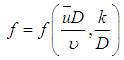 | (7) |
Thus for the laminar type flows determined by  , the shear factor is defined as dependent only on the Reynolds number:
 | (8) |
To the flows with  , called turbulent, are presented divided in three types whose shear factor is expressed individually in each one, as:1. Turbulent hydraulically smooth with
  , and “f” modeled by:
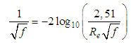 | (9) |
2. Turbulent hydraulically rough, with  , and “f” modeled by:
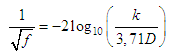 | (10) |
3. Turbulent hydraulically mixed, with 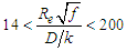 , and “f” modeled by the Colebrook/White expression:
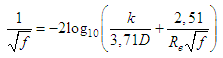 | (11) |
[5], [6].
4. Modifications and Adaptations of the Equations
The Eq. 8 has origin from the Louis Marie Henri Navier and George Gabriel Stokes studies, in the second half of the XIX century, which identified the presence of molecular forces in the fluid mass and admitted that in a permanent and fully developed flow the existence of tensions causes deformations that are defined by the velocity spatial variations, and the Eqs. 9, 10 e 11 were obtained based on the velocity distribution model proposed by Von Kármán-Prandtl in the beginning of the following century [5, 6].Despite of the consolidated success in the use of these three equations for the determination of the shear factor in turbulent flows, it is opportune to describe in detail its conceptual "inconsistencies", where basically the expressions used to estimate “f” were conceived on the basis of a model of Velocity distribution that presents inaccuracies in three main characteristics: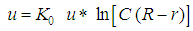 | (12) |
when “ ”, at the water-tube interface,
  , which characterizes a limitation of this speed distribution.1. Another weakness of this equation is the lack of a mathematical formulation for estimates of the shear factor when the Reynolds number occurs in the interval between (2500 and 4000), transition region between laminar and turbulent flow regimes.2. In addition, in the center of the tube, where
  , the derivative “
 ” is different of zero, implying a shear stress is other than zero, where physically it should be null. The application of the probability concepts in hydraulic of flows, initiated by Chao Lin Chiu in 1987, resulted in the attainment of a new equation for the distribution of velocities, therefore improving the mathematical modeling of this physical occurrence. Under a new optic, this new approach allowed the determination of the shear tension model; the in suspension sediments concentration model; and the profiles determination model of transversal sections in rivers and open channels [1, 2].Once developed the expression describing the distribution of velocities in flows, Chiu in 1993 also presented a new mathematical formulation to better model the shear factor, “f”, based on a more realistic velocity distribution model, and thus overcome the deficiencies presented by the classical distribution law, Eq. 12, and represents for Hydraulic Engineering an important advance, for continuing to solve well the challenges by the flows under the pressure, and also because it generalizes the equations enlarging the horizon for the mathematical modeling workers in Hydraulics [6, 7].This new distribution, in turn, proves to satisfy both free flow and flow under pressure, and the coordinate “
 ”, when for a circular cylindrical tube, takes the form
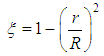 | (13) |
In the tube axis, where “ ", “
", “ ” and “
 ” are present, and at the interface water-tube, where “
 ”, “
”, “ ” and “
 ” are used. Thus, the final form of velocity distribution in forced ducts formulated by this author in 1993, takes the form:
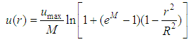 | (14) |
This equation indicates that for “ ” (at the interface water-pipe), we have “
 ”, and for “
 ”, in the tube axis, we have “
 ”, and another interesting result resulting from this distribution, is the average velocity in the section, as another interesting result due to this distribution expressed by the author for:
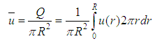 | (15) |
with u(r) given by Eq. 14 which and that implies in the important result: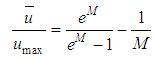 | (16) |
The entropy parameter “M” univocally defines the ratio between “ ”, and can to vary from zero (laminar flow) up to infinity, a value at which the velocity distribution becomes uniform, in other words, which “
 ”.When the right side of Eq. 16 is analyzed for, this member has a limit of 1/2 indicating that "" which reveals a classic result for laminar flow in a circular cylindrical tube, Figure 1. For, however, the limit of Second member is equal to 1, indicating that in this condition "", confirming the fact that the velocity distribution profile tends to a uniform geometry as there is an increase in the degree of turbulence of the flow and consequently of the parameter “M”, given to the increase in Reynolds number.
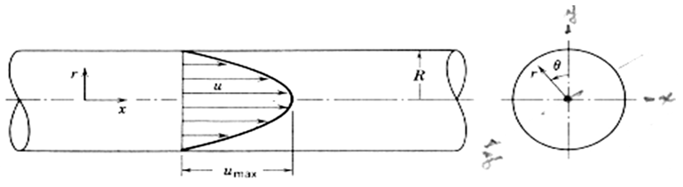 | Figure 1. One-dimensional laminar flow in pressurized duct |
The “ f ” factor obtained based on the new distribution of velocities was established by Chiu from the generalization of the Newton law for viscosity, valid only for laminar flow and that relates the shear tension with the transversal gradient of velocity. Chiu proposed the same relation between these magnitudes for the turbulent flow condition and that, when applied to the interface fluid-pipe, acquires the form: [1, 2].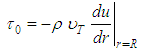 | (17) |
Where “ ” is the turbulent viscosity and understood as a property of the flow regime state of turbulence, and not only as a molecular property of the fluid. In this way, in the regions not affected by the flow turbulence we understand that “
 ”. With the gradient “
 ” obtained from the distribution “
 ”, Eq. 14 can be written:
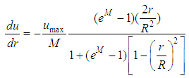 | (18) |
in which for “ ”, is transformed in:
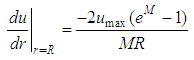 | (19) |
This result, when substituted in Eq. 17, expresses the shear tension close to the pipe internal wall as: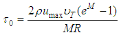 | (20) |
From this Eq.20, and knowing the relation given by Eq. 2, Chiu expresses “ ” by:
” by: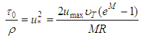 | (21) |
Multiplying “ ” in both members of the Eq. 21, and replacing “
 ” by “
 ”, it has been:
 | (22) |
which the inverted form is expressed as: | (23) |
Knowing that: | (24) |
and that the ratio between the maximum and average speeds is: | (25) |
and further, defining Reynolds in the state of full turbulence as: | (26) |
and, yet, replacing “ ” from Eq. 23, “
 ” from Eq. 25 and “
 ” from Eq. 25 into Eq. 24, Chiu, in 1993, obtained a new expression for the shear factor:
 | (27) |
which written in a more compact form becomes: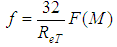 | (28) |
being: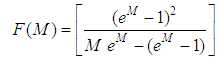 | (29) |
[2].
5. The Validation of the Entropic Model
The validation and consistency of the expression, Eq. 27, can be checked by the identification and performance of the entropy parameter, “M”, in the classical flow regimes, as known, based on the velocity distribution studies of Von Kármán-Prandtl§ Laminar flow: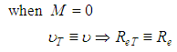 For “M = 0”, the limit of , from Eq. 29, after the use of the L'Hospital rule, is equal to 2, from which the classical expression of the shear factor for laminar flows is obtained:
 § Turbulent flow hydraulically smooth:In this type of flow, the conditions under which,
  and
and  within the viscous sublayer, adjacent to the wall where
  , where the friction factor is expressed by:
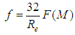 As in the hydraulically smooth turbulent flow the factor “f” is dependent only on the Reynolds number, it becomes evident from Eq. 28 that the entropy parameter “M”, is also consequently dependent only on the Reynolds number.§ Turbulent flow hydraulically rough:In this type of flow, in turn, there is no region (even adjacent to the wall) without turbulence, which validates the assertion that
  , such that “f” is expressed by
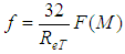 For this case in particular, due to the flow nature, it is known that the shear factor must depend on only the relative roughness “
 ” what allows the affirmation that both “
 ” and “M” depend only on “
 ”, Eq. 27. § Turbulent flow hydraulically mixed:For this particular case, by the nature of the flow, it is known that the shear factor should only depend on the relative roughness “
 ”, which allows the assertion that both “
 ” and “M” also depend only on “
 ”.It is also possible to state that, for a hydraulically mixed flow, the parameter “M” must depend on both “
 ” and “
 ” and, additionally, the factor “f” in these conditions also expresses the same dependencies, proving univocal in relation to the entropy parameter “M”.
6. The Numeric Adjustment
At this point, the process developed by Chiu has been narrated up to here, it is evident the discomfort in the handling of Eq. 27, given the presence of the parameter “M” and the number of turbulent Reynolds “ ”, two variables that are difficult to obtain in practice.In this way, by adding considerations to the mathematical treatment of Chao Lin Chiu involving the shear factor, this project insists on the relevance of knowing a conjecture that represents well the velocity distribution, already referenced by Kárman and Prandtl, as:
 | (30) |
where the maximum, medium and shear velocities,  , respectively, are related for any flow in turbulent regime. [2], [4].On the other hand, in addition to knowing that other different values for the multiplying constant, such as 3.75 and 4.07, can be found in the literature, it is therefore pertinent to look at the fact that physically, it is more important to know of the existence of a constant that multiplies “
 ”, and which validates Eq. 30, than the knowledge of the value of the constant itself. This is because in knowing that there is a constant in the expression, experimentally, it is possible to approximate its value.Therefore, in this aspect, it can be conjectured the existence of a universal constant “C” satisfying the condition below, valid only for turbulent flows.
 | (31) |
and the value of this constant can be explicit as: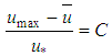 | (32) |
Making use of the relation among  ,
,  and M, described by Chiu in the Eq. 25, we have:
 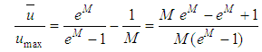 | (33) |
from where it can be obtained: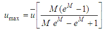 | (34) |
Subtracting form the two members of Eq. 34 the value of “ ” and then dividing both the members by “
 ”, the following relation is obtained:
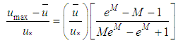 | (35) |
Such as in Eq. 31, the first member of Eq. 35 is equal to “C”, and being the ratio  of the second member equal to
  . The Eq. 34 is transformed in:
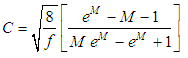 | (36) |
In this way, the Eq. 36 can be rewritten as an expression generalized for the calculation of the “f” shear factor, dependent only on the parameter “M”, as: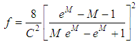 | (37) |
Here, it is important to stress that the universal constant “C” value deserves to be experimentally better exploited, making room to developments that explore better the velocities profile in these flows. Since this exploration goes beyond the scope of this work, it is suggested the adoption of the value described by Hunter Rouse in “Elementary Mechanics of Fluids” in 1946, with C = 4,045, that substituted in the Eq. 37, provides the expression for “f”, as: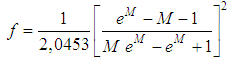 | (38) |
This model is undoubtedly more complete than the traditional one deducted from the logarithmic velocities distribution, classically used in the universal formula of the distributed load loss in forced pipe. However, it brings yet with it self the same limitations and discomforts of the formulation presented by Chiu for the shear factor with the Eq. 27, that in spite of being unique and generic, with application both to laminar flows and to any turbulent flow, it also has the turbulent Reynolds explicit presence defined as: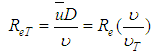 and the use of the “M” entropy parameter as “
 ”, where “
 ” is one of the Lagrange multipliers used in the maximization operation.At first, Eqs. 27 and 38 enable the “M”, parameter elimination and also the attainment of a formulation for the “friction” factor that is dependent only on “
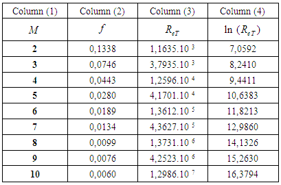
 ”, what already would translate the big advance due to the existence of a single parameter in the equation for the “f”. calculation. However, the algebraic structure of these equations revealed, after several attempts, an analytical “impossibility” for the elimination of the parameter, reason for which the use of a mathematical adjustment by minimum squares was chosen in the discard of this variable [1, 3].The task of “M” elimination, by adjustment, was preceded by the Table 1 assembly, following the order:§ Values for “M = 2,3,…,10” were adopted forming the column 1;§ With the adopted “M”, values, the correspondent “f”, values were calculated trough Eq. 38 generating the column 2; § With the “M” and “f”, values, the attainment of the respective “
 ” values was possible, with the use of Eq. 27, forming the column 3;§ The
  values were placed at column 4.
Table 1. Values of
 for turbulent flows for turbulent flows
 |
| |
|
In a first moment, and with the objective of determining a third expression that best relates the equations 27 and 38 trough the discard of the entropy parameter, the adjustment was sought with the help of an EXCEL sheet among the “f” values (column 2) and the “ ” turbulent Reynolds values (column 3), that after several attempts showed incongruent results. It denounced these responses inconsistency as characteristics inherent to the adjustments among very small numbers (shear factor) and very large numbers (turbulent Reynolds). This lead to new attempts for the adjustment among more coherent values correlating thus “f” and “
 ” (column 4), revealing an equation with determination index
  , represented in the form:
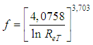 | (39) |
Such as Eq. 38, this equation is applicable only to the turbulent type flows. Because of that, it is conclusive to affirm that, in the case of hydraulically smooth turbulent flow, whenever the viscous sub layer overcomes the hydraulic roughness “k” we have the condition “ ” close to the pipe wall, what reduces “
 ” (turbulent) to “
 ” (usual) and, in these conditions, the Eq. 38 acquires the form:
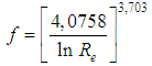 | (40) |
Hence, once the proposal represented by the conjecture “ ”, is accepted, the theory of maximum entropy allows the obtaining of the Eq. 40, for the “f” determination, in the hydraulically smooth turbulent flow condition, without the need of any experiments.In the other turbulent flow conditions, hydraulically rough or mixed, the Eq.39 should allow the shear factor determination if the turbulent Reynolds number, “
 ”, is a known value. Since the relation between
  and
and  is given by
  , the determination of “
 ” comes from the “
 ” knowledge and, with more difficulties, from the ratio between the molecular viscosity and the “
 ” turbulent viscosity.In this way, the hydraulically rough turbulent flow corresponds to a limit condition that occurs for big values of the dimensionless “
 ”. At this point then, the shear factor starts to depend only on the hydraulic roughness relative to the pipe diameter “
 ”. In this flow regime condition, the “k” roughness value is much superior to the viscous sub layer thickness, making the extremities of the pipe wall imperfections, whose roughness composes “k”, as the only source responsible for the turbulence generation, as Figure 2 illustrates.
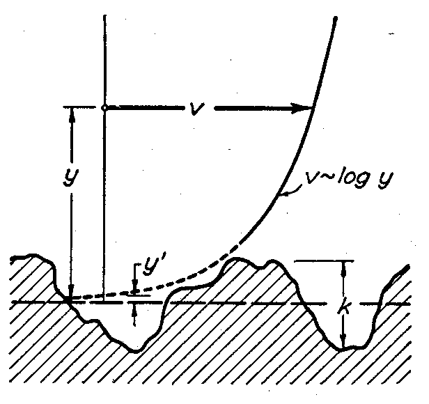 | Figure 2. Representation of the internal walls imperfections of a generic pipe. The imperfections are bigger than the limit |
Under these circumstances, in hydraulically rough turbulent flow, the dependence between the “f” factor and the relative roughness of the pipe “ ” is known. This relation was established at first from the classical experience of Johan Nikuradse, that involved roughnesses produced by “uniform” sand grains, internally fixed to the pipes walls, with previously known diameters, with the “
 ” values equal to 30; 61,2; 120; 252; 504; 1014 and relating them with the correspondent “f” factor values, through the expression
 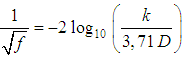 , Eq. 10, [6, 7]If in this hydraulically rough turbulent flow condition the shear factor is dependent only on “
 ”, as above mentioned, it is reasonable that the Eq. 39 is kept valid and becomes to be rewritten with a algebraic structure closer to mathematical relations traditionally known for the “f ”, as:
 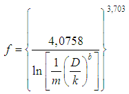 | (41) |
or in the form: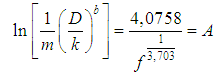 | (42) |
where the “b ” exponent and the “m” coefficient must be determined so that the Eq. 41 represents the best Nikuradse data as possible. From a generic manner it is still possible to write the Eq. 41 as: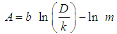 | (43) |
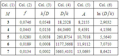
As described in the previous proceeding, the numerical adjustment of magnitudes present in this “A ” expression and “ ” allows the “b” and “m” values determination and reveals the first analytical structure for the “f” presented by this project trough the Eq. 41. For this, also trough the same process previously described, it followed the Table 2 assembly, with the following itemization:§ Values of “
 ” that are in column 1, were adopted; § With the adopted “M ” values, the correspondent “f” values were calculated trough Eq. 38, that form the column 2; § These “f” values allowed the determination of the “
 ” values, with the use of Eq. 10, whose results are in the column 3;§ In the column 4 are located the values of
 ;§ In the column 5 are the “A” values, defined by Eq. 42 and calculated from the “f ” factor of column 2.§ In the column 6 are the values of “
 ”.
”.Table 2. Values of
 for hydraulically rough turbulent flows for hydraulically rough turbulent flows
 |
| |
|
In this way, with the use of the EXCEL sheet, the adjustment of the curve generated for  (column 5) was achieved, and
  (column 6), attaining an equation that represented a
  determination index, and with the
  structure, that whenever equaled to Eq. 42, provides the
  .
.
7. Conclusions
Finally, the suggested formula for the shear factor determination in hydraulically rough turbulent flows, based on the distribution of velocities, derived from the Maximum Entropy principle is: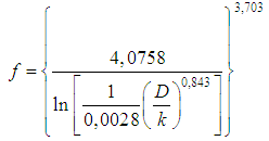 | (44) |
In the hydraulically mixed turbulent flow condition, the shear factor can be determined by an expression that contains the arguments of the hydraulically smooth turbulent flow regime, Eq. 40, and of the hydraulically rough turbulent, Eq. 44, following exactly the 1937 Colebrook-White suggestions that enable to write the expression that best represents this flow regime as: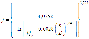 | (45) |
It is relevant to stress that the Eq. 44 presents asymptotic behaviors revealing that, whenever , it is transformed in the Eq. 44. It translates a flow regime with dependencies only on the roughness relative to the pipe diameter, identified as hydraulically rough turbulent. On the other hand, whenever
  , the Eq. 44 stays reduced to Eq. 40, valid to the flow regime dependent only on the Reynolds number, translating a hydraulically smooth turbulent regime. Therefore, restructuring the expression for the “f” factor calculation, that identifies a hydraulically mixed flow regime, it can be presented better as:
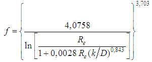 | (46) |
Moreover, from the comparison between this equation 45 and the Eq. 38 and, also, knowing that 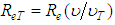 , an expression for the “
 ” ratio between the turbulent and molecular viscosities is obtained, as:
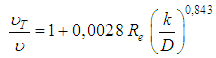 | (47) |
This expression, Eq. 46, is shown to be coherent with the forced flow physical mechanism, since whenever the “k” roughness is null, or insignificant, we have “ ”. It is therefore a fact that characterizes the hydraulically smooth turbulent flow occurrence, where “
 ”.Likewise, it is evident the need to work in future researches on the validation and consistence of the conjecture expressed by Eq. 31, in which “C ” is proven constant, followed by a posterior determination of its value. It is fundamental for the advance in the treatments with the mathematical modeling in the permanent and fully developed flows in pressurized ducts.
References
| [1] | CHIU, C. L. Application of entropy concept in pipe flow study. Journal of Hydraulic Engineering, v. 119, n. 6, p. 742-756, June 1993. |
| [2] | CHIU, C. L. Entropy and 2D velocity distribuition in open channel. Journal of Hidraulics Engineering, v. 114, n. 7, p. 738-756, July 1988. |
| [3] | GOLDMANN, S. Information teory. 3. ed. New York: MacGraw-Hill, 1953. 385p. |
| [4] | JELINEK, F. Probabilistic infomation theory – discret and memory less models. New York: MacGraw-Hill, 1968. 609p. |
| [5] | LENCASTRE, A. Hidráulica geral. Lisboa, Edgard Blücher Ltda., 1983. 411p. |
| [6] | ROUSE, H. Elementary mechanics of fluids. New York: John Wiley, 1946. 376p. |
| [7] | SHULZ, E.H. Alternativas em turbulência. São Carlos: ESSC/USP, 2001. 140p. |

 Abstract
 Reference
 Full-Text PDF
 Full-text HTML