Alexandre Beluco, Edith Beatriz Camano Schettini
Instituto de Pesquisas Hidráulicas (IPH), Universidade Federal do Rio Grande do Sul (UFRGS), Porto Alegre, Brazil
Correspondence to: Alexandre Beluco, Instituto de Pesquisas Hidráulicas (IPH), Universidade Federal do Rio Grande do Sul (UFRGS), Porto Alegre, Brazil.
| Email: |  |
Copyright © 2016 Scientific & Academic Publishing. All Rights Reserved.
This work is licensed under the Creative Commons Attribution International License (CC BY).
http://creativecommons.org/licenses/by/4.0/

Abstract
The solution of the Colebrook White equation continues to attract the attention of engineers and mathematicians. Some solutions proposed in recent years have two or more internal iterations and present relative complexity. At the same time, micro-computers and calculators have shown increased calculation capacity, virtually eliminating approximations that have a certain accuracy but that are too complex. A direct approximation of the equation allowing for quick and accurate solution is still useful. This technical note brings together some explicit approximations with only one internal iteration presented in the 1970s and 1980s into a single category and proposes a single model with five parameters to be determined. Moreover, this technical note also presents the values for these five parameters that minimize the mean square error related to the outcome of the Colebrook White equation, considered as a reference. The proposed model allows to obtain results with mean square error equal to 1.14 x 10⁻⁸, with maximum relative error of 4.44% and 96.78% of results below 1.00% of difference relative to Colebrook White equation, which can be considered quite satisfactory.
Keywords:
Friction factor, Energy loss in pipes, Colebrook White equation
Cite this paper: Alexandre Beluco, Edith Beatriz Camano Schettini, An Improved Expression for a Classical Type of Explicit Approximation of the Colebrook White Equation with Only One Internal Iteration, International Journal of Hydraulic Engineering, Vol. 5 No. 1, 2016, pp. 19-23. doi: 10.5923/j.ijhe.20160501.03.
1. Introduction
The Colebrook White equation was proposed [1] in 1937 and its non-algebraic characteristic, hindering its solution, still attracts the attention of engineers and mathematicians. Moody [2] proposed a diagram containing all the information summarized in the equation and serving as an abacus for determining the friction factor f.During the 70s and 80s, the first approximations to the equation of Colebrook White, basically with only one internal iteration have been proposed. The first personal computers became popular, but still showing inability to solve the Colebrook White equation in problems involving the calculation of a large number of pipes.During the following decades, several other approximations have been proposed, with increasing complexity, some with two or three [3] or even more internal iterations and others with different shapes or different methods [4] of the structure proposed by Colebrook and White.Currently, the Colebrook White equation can be solved by personal computers and even an exact although complex solution was proposed [5, 6]. Even with great accuracy [7, 8], the evolution of computers reduces the usefulness of approximations with high computational costs.Currently, there is a large number of papers proposing alternative equations to the expression proposed by Colebrook White, with different shapes and several of them with better results for a particular type of flow [9, 10] or for a certain type of fluid [11]. This paper presents an equation with scope and applicability equivalent to the original expression, therefore suitable for Newtonian fluids and turbulent flows, for a wide range of roughness values.An approximation of the Colebrook White equation that represents a computational cost equivalent to only one iteration and displays reasonable accuracy could still be applied to calculations of large pipe networks.This technical note includes six classical approximations of the Colebrook White equation with a similar shape in a same category. These approximations have been proposed in the 1970s and 1980s and have computational cost equivalent to one internal iteration.This technical note also proposes a generic model for this category, with five parameters to be determined so as to minimize the difference of their results with the Colebrook White equation, considered as reference in this study.Finally, this technical note provides values for these five parameters so that the model proposed to provide better results than those obtained with the six models taken as the starting point.
2. The Friction Factor and the Colebrook White Equation
The friction factor f appears in the Darcy equation for energy loss in pipes. The factor f is dimensionless and depends on the pipe diameter, roughness of the material of the pipeline and the Reynolds number of the flow.Darcy's equation for the calculation of the loss of pressure hP [m] is shown in Eq. (1) where L [m] is the tube length considered in the calculation, D [m] is the pipe diameter, V [m/s] is the speed and g [m/s2] is the acceleration of gravity. | (1) |
The friction factor can be calculated for turbulent flow by the Colebrook White equation. It is a non-algebraic equation with iterative resolution. The Eq. (2) shows the typical presentation of this equation, where e [m] is the roughness of the pipe and Re [1] is the Reynolds number. e/D [1] is the relative roughness.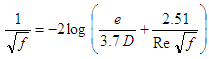 | (2) |
Eq. (3) directly indicates the value of f after each iteration. The initial value used in the iterations can reduce the amount of calculations, but the process usually converges to a reasonable accuracy after a few iterations.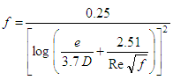 | (3) |
Good accuracy in result is already obtained with few iterations. For simple calculations, it is not interesting to adopt approaches to this equation. The use of approximations that directly provide the final value, even with a loss of precision, will be interesting for the design of networks with large numbers of tubes.
3. Some Classical Basic Approximations of the Colebrook White Equation
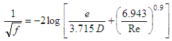
Several approximations for the Colebrook White equation have been proposed in last decades and they are still being proposed. The trend that can be expected from new approaches is that they will present lower computational costs. Among them, one interesting class can be established for the approximations with only one internal iteration and similar constitution to the Colebrook White equation.This class would include the equations proposed by Haaland [12], Barr [13, 14], Jain [15], Swamee and Jain [16], Churchill [17] and Eck [18]. Eq. (4) shows the equation proposed by Haaland [12]. According to Winning and Coole [19], this equation provides results with a maximum percentage relative error of 1.43% and MSE equal to 2.67 x10⁻⁸.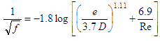 | (4) |
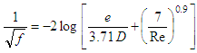
Eq. (5) shows the equation proposed by Barr [13, 14] and Eq. (6) shows the equation proposed by Jain [15].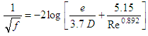 | (5) |
 | (6) |
Eq. (7) shows the equation proposed by Ref. [16] and Eq. (8) shows the equation proposed by Churchill [17].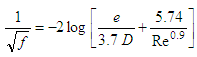 | (7) |
 | (8) |
Eq. (9) shows the equation proposed by Eck [18].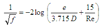 | (9) |
These equations can be generalized to a model with five parameters, aiming to optimize these parameters to reduce the error in relation to the Colebrook White equation. The next section discusses a model developed in this way.
4. A Model for an Explicit Approximation with Only One Internal Iteration
It is possible to build a generic model for this class of explicit approximations containing five variables to be optimized, thereby reducing the error in relation to the Colebrook White equation. Eq. (10) shows the proposed model. Comparing the expressions (4) to (9), changes were observed in five locations on the basic structure of the Colebrook White equation.The five variables together must compensate for the withdrawal of the factor f from the inside of the logarithm. Z is a factor external to the logarithm function. A and B respectively integrate the terms including roughness and Reynolds number. The exponents a and b do not appear in the original structure proposed by Colebrook and White.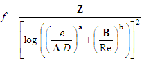 | (10) |
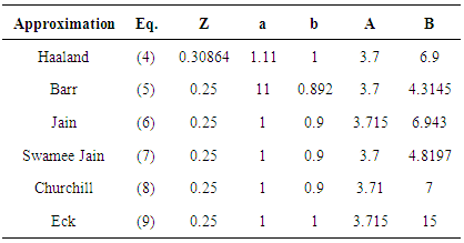
Table 1 shows the values of the five parameters of the model of Equation (10) corresponding to the approaches presented in previous section.Table 1. Parameters for the model of Eq (10)
 |
| |
|
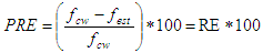
The proposition of this model aims to obtain a model that is more accurate than the six approximations mentioned above. In other words, it is necessary to find values for the parameters Z, a and b, A and B that achieve f values more accurately than those provided by equations (4) to (9).The accuracy of the approximations can be evaluated by the relative error and the mean square error. Eq. (11) and (12) define respectively the relative error (RE) and the percentage relative error (PER) and Eq. (13) establishes the mean square error (MSE), where fcw is the value provided by the Colebrook White equation and fest is an estimation obtained with equations (4) to (9) or with the model in Eq. (10).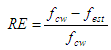 | (11) |
 | (12) |
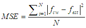 | (13) |
this work, the results provided by the Colebrook White equation, solved for a large number of iterations, were considered as reference. The friction factor fcw were obtained with 16 iterations and were considered as reference for comparison with other models. From the calculations with the Colebrook White equation and the model of Eq. (10), the relative error and mean square error were determined.The calculations were performed for 46 values of the relative roughness and 52 values of Reynolds number. The values of the relative roughness were 0.09, 0.08, 0.07, 0.06, 0.05, 0.04, 0.03, 0.02, 0.01, 0.009, 0.008, 0.007, 0.006, 0.005, 0.004, 0.003, 0.002, 0.001, 0.0009, 0.0008, 0.0007, 0.0006, 0.0005, 0.0004, 0.0003, 0.0002, 0.0001, 0.00009, 0.00008, 0.00007, 0.00006, 0.00005, 0.00004, 0.00003, 0.00002, 0.00001, 0.000009, 0.000008, 0.000007, 0.000006, 0.000005, 0.000005, 0.000003, 0.000002, 0.000001 and 0.The values of Reynolds number were 3.0x10³, 4.0x10³, 5.0x10³, 6.0x10³, 7.0x10³, 8.0x10³, 9.0x10³, 1.0x10⁴, 2.0x10⁴, 3.0x10⁴, 4.0x10⁴, 5.0x10⁴, 6.0x10⁴, 7.0x10⁴, 8.0x10⁴, 9.0x10⁴, 1.0x10⁵, 2.0x10⁵, 3.0x10⁵, 4.0x10⁵, 5.0x10⁵, 6.0x10⁵, 7.0x10⁵, 8.0x10⁵, 9.0x10⁵, 1.0x10⁶, 2.0x10⁶, 3.0x10⁶, 4.0x10⁶, 5.0x10⁶, 6.0x10⁶, 7.0x10⁶, 8.0x10⁶, 9.0x10⁶, 1.0x10⁷, 2.0x10⁷, 3.0x10⁷, 4.0x10⁷, 5.0x10⁷, 6.0x10⁷, 7.0x10⁷, 8.0x10⁷, 9.0x10⁷, 1.0x10⁸, 2.0x10⁸, 3.0x10⁸, 4.0x10⁸, 5.0x10⁸, 6.0x10⁸, 7.0x10⁸, 8.0x10⁸ and 9.0x10⁸.The determination of the values of the five parameters of the model of equation (10) to minimize the RE and MSE values can be performed with the Matlab software. The ER and MSE values were obtained for the values of Z between 1 and 2, a between 1 and 2, A between 1 and 2, b between 1 and 2 and B between 1 and 2.The next section presents and discusses the results.
5. Results and Discussion
The MSE minimization of the five parameters resulted in the following values: Z=0.30091, A=1.09540, B=0.969491, a=3.73150 and b=5.98017. These values may be rounded to the fourth decimal with no significant change in accuracy of the results, as shown in Eq. (14).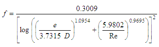 | (14) |
This equation is the best result of this work, with a maximum relative error of 4.44% and MSE equal to 1.14 x10⁻⁸. Among the values of relative roughness and Reynolds numbers used in the calculation, 92.60% are lower than the percentage relative error of 0.08% and 96.78% are lower than PRE of 1.00%. Figure 1 shows the relative error distribution to the ranges of relative roughness and Reynolds number considered.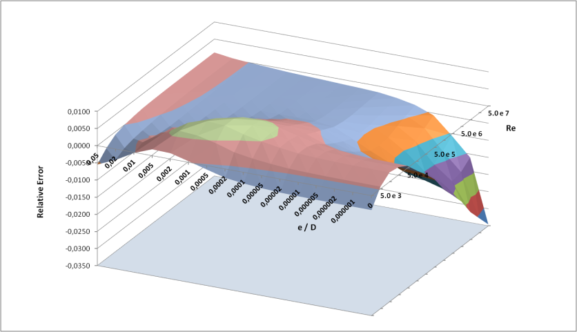 | Figure 1. Relative error of the proposed model shown in Eq. (13) |
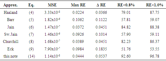
Table 2 shows a comparison between the MSE for the classical equations and the MSE obtained for the equation proposed in this paper. This table also shows maximum values of RE, difference between negative and positive maximum values of RE and percentage of values of RE lower than 0.08% and lower than 1.00%. The equation of this paper is the best approximation when compared with the classical equations discussed in previous section.Table 2. Comparison of results with Eq. (14)
 |
| |
|
Table 2 shows that the proposed equation has the lowest MSE and the greatest number of results with relative error less than 0.8% and less than 1.0%. The low MSE value makes the surface appearing in Figure 1 "flatter" than the surfaces corresponding to other approximations and allows a greater amount of values with less difference with respect to the Colebrook White equation.
6. Conclusions
This technical note included six classical approximations of the Colebrook White equation in a same category and also proposed a generic model for this category, with five parameters to be determined. These five parameters were determined, presenting a new alternative equation with only a single iteration with RMSE equal to 1.125x10⁻⁸.
References
| [1] | Colebrook, C.F.; White, C.M.; 1937. Experiments with fluid friction in roughened pipes. Proceedings of the Royal Society of London, Series A, 161, p.367-381. |
| [2] | Moody, L.F.; 1947. An approximate formula for pipe friction factors. Transactions of the ASME, 69 (12), p.1005-1006. |
| [3] | Romeo, E.; Royo, C.; Monzón.; 2002. A. Improved Explicit equations for estimation of the friction factor in rough and smooth pipes. Chemical Engineering Journal, 86, p.369-374. |
| [4] | Ozger, M.; Yildirim, G.. 2009. Determining turbulent flow friction coefficient using adaptive neuro fuzzy computing technique. Advances in Software Engineering, 40, p.281-287. |
| [5] | Sonnad. J.R.; Goudar, C.T.; 2004. Constraints for using Lambert W function based explicit Colebrook White equation. Journal of Hydraulic Engineering, 130, p.929-931. |
| [6] | Sonnad, J.R.; Goudar, C.T.; 2007. Explicit reformulation of the Colebrook White equation for turbulent flow friction factor calculation. Industrial & Engineering Chemistry Research, 46, p.2593-2600. |
| [7] | Yildirim, G.; 2009. Computer based analysis of explicit approximations to the implicit Colebrook White equation in turbulent flow friction factor calculation. Advances in Software Engineering, 40, p.1183-1190. |
| [8] | Brkic, D.; 2011. Review of explicit approximations to the Colebrook relation for flow friction. Journal of Petroleum Science and Engineering, 77, p.34-48. |
| [9] | Shaikh, M.M.; Massan, S.T.; Wagan, A.I.; 2015. A new explicit approximation to Colebrook’s friction factor under rough pipes under highly turbulent cases. International Journal of Heat and Mass Transfer, 66, p.538-543. |
| [10] | Brkic, D.; 2016. A note on explicit approximations to Colebrook’s friction factor in rough pipes under highly turbulent cases. International Journal of Heat and Mass Transfer, 93, p.513-515. |
| [11] | Dosunmu, I.T.; Shah, S.N.; 2013. Evaluation of friction factor correlations and equivalent diameter definitions for pipe and annular flow of non-Newtonian fluids. Journal of Petroleum Science and Engineering, 109, p.80-86. |
| [12] | Haaland, S.E.. 1983. Simple and explicit formulas for friction factor in turbulent pipe flow. Journal of Fluids Engineering (ASME), 105 (1), p89-90. |
| [13] | Barr, D.I.H.; 1972. New forms of equations for the correlation of pipe resistance data. Proceedings of the Institution of Civil Engineers, 53 (2), p.383-390. |
| [14] | Barr, D.I.H.; 1981. Solutions of the Colebrook White function to resistance to uniform turbulent flow. Proceedings of the Institution of Civil Engineers, 71 (2), p.529-535. |
| [15] | Jain, A.K.; 1976. Accurate explicit equations for friction factor. Journal of the Hydraulic Division (ASCE), 102 (5), p.674-677. |
| [16] | Swamee, P.K.; Jain, A.K.; 1976. Explicit equation for pipe flow problems. Journal of the Hydraulic Division (ASCE), 102 (5), p.657-664. |
| [17] | Churchill, S.W.; 1973. Empirical expressions for the shear stressing turbulent flow in commercial pipe. AIChE Journal, 19 (2), p.375-376. |
| [18] | Eck, B. Technische Stromungslehre. Springer, New York, United States, 1973. |
| [19] | Winning, H.K.; Coole, T.; 2013. Explicit friction factor accuracy and computational efficiency for turbulent flow in pipes. Flow, Turbulence and Combustion, 90, p.1-27. |

 Abstract
 Reference
 Full-Text PDF
 Full-text HTML