Nasreddine Meziane1, Ahmed Bettahar2, M’hamed Beriache2
1Hydraulic Department, Faculty of Civil Engineering and Architecture, University Hassiba Benbouali of Chlef, Chlef, Algeria
2Mechanical Engineering Department, Faculty of Technology, University Hassiba Benbouali of Chlef, Chlef, Algeria
Correspondence to: Nasreddine Meziane, Hydraulic Department, Faculty of Civil Engineering and Architecture, University Hassiba Benbouali of Chlef, Chlef, Algeria.
| Email: |  |
Copyright © 2015 Scientific & Academic Publishing. All Rights Reserved.
This work is licensed under the Creative Commons Attribution International License (CC BY).
http://creativecommons.org/licenses/by/4.0/

Abstract
The objective of this work is to propose a new approach to dimensioning of the conduits partially or totally filled. To dimension the conduit, the wetted section and the wetted perimeter have to be expressed under the forms  and
and  . The study is based on the relationships universally known of the Darcy-Weisbach and of Colebrook-White. In this study, the new developed approach leads to an explicit solution and the ensuing results can be compared to the different exiting models. The maximum relative error obtained of the 80% calculated values does not exceed 0.25%. What enables us to say that this approach adapts well to manual and computing calculations. It was found that this new contribution is more accurate than the most equations available literature.
Keywords:
Dimensioning, Conduit partially filled, Conduit totally filled, Explicit relationship, Conduit diameter
Cite this paper: Nasreddine Meziane, Ahmed Bettahar, M’hamed Beriache, High Accurate Explicit Solution for the Determination of Conduit Height, International Journal of Hydraulic Engineering, Vol. 4 No. 4, 2015, pp. 95-102. doi: 10.5923/j.ijhe.20150404.02.
1. Introduction
Flow in a conduit partially or totally filled is governed by a functional relationship of type  where Q is the volume flow rate, J is the hydraulic slope in a section of the conduit or of the channel of length
  is the hydraulic diameter,
  is the absolute roughness of the conduit wall and
  is the filling rate. The dynamic viscosity
  and density of the fluid
  being known, so as the length
  of the conduit and its absolute roughness
  (depending on the used material). Three types of problems occur: I-Determine the hydraulic slope J of the conduit knowing its diameter and an imposed volume flow. II-Determine the volume flow Q in the conduit knowing its diameter and a hydraulic slope imposed. III-Determine the hydraulic diameter
  or geometric diameter of conduit D knowing the volume flow at ensure under an imposed hydraulic slope. In turbulent flow, the hydraulic slope is more or less exactly proportional to the square of the velocity (respectively volume flow rate). Also, the shear stress at the wall
  (for a noncircular cross section its mean value) is equal to
  , where
  is a number depending on the particular conditions and mainly of the wall roughness, and
  is the mean velocity. The hydraulic slope in a section of conduit or of the channel of length
  must ensure the equilibrium of the tangential tensions at the wall surface. Therefore, v, J and
  are related by the well-famous equation of Darcy [6] Rel. (1), that, applied to a conduit partially or totally filled, is written in the form:
 | (1) |
According to the classification of the problems in the field of practical calculation of the conduits cited above, the problem of type III is the most frequently encountered in engineering problems (full circular pipe), and also the most difficult to solve. The general law of the linear load loss coefficient of Colebrook [5] Rel. (2) has an algebraic form which often leading to numerical calculations by iteration. Therefore, we use more frequently the graphic methods based on the use of the Moody diagram (Moody 1947).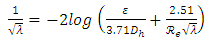 | (2) |
The solution of the problems of type II and III is much more delicate since the available data don’t allow the initial calculation of the Reynolds number, nor that of the relative roughness in problem III. Jain, Swamee and Jain [17], Haaland [10], Imbrahim [12], Valiantzas [22], Diniz and Souza [7], Brkić [4], Giustolisi et al [8] and Li et al. [14] have established explicit relationships applicable to the first category of problems. For the second category of problems, an explicit solution was proposed by Hager [11] and Sinniger and Hager [16]. Regard to the third category of problems, approximate solutions have been proposed by certain authors for the resolution of the basic equation system of a turbulent flow in circular conduit in charge. Among the most significant studies those of Swamee and Jain [17, 18, 19], of Swamee and Rathie [20], of Swamee and Swamee [21], of Hager [11], of Bedjaoui and Achour [3], of Babajimopoulos and Terzidis [2], of Gulyani [9], of Bombardelli and Garcia [3] and Achour et al. [1]. The latter authors showed that their study can be adapted to any form of conduits or channels in charge or open channel flow.
2. Geometric Properties
Considering the Fig.1 for a flow section of given geometric form: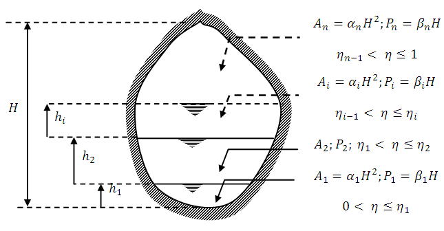 | Figure 1. Flow section composed of n zones |
Either: are respectively, the wetted section, the wetted perimeter, the maximum filling ratio of the zone of rank i and the height of the conduit.Also:
 are respectively, the relative coefficient of the wetted section, the relative coefficient of the wetted perimeter and the maximum water height of the zone of rank i. The formulas presented below are to perform the calculation of geometric elements at one and three depth zones of some usual cross-sections: Table 1 oval section, Table 2 horseshoe section and Table 3 circular section.Ovoid sectionTable 1 presents the formulas of geometric elements of an ovoid section composed of three zones of heights.
 Table 1. The calculation formulas of geometric elements of three depth zones of an ovoid section
 |
| |
|
Horseshoe cross sectionTable 2 presents the formulas of geometric elements of a horseshoe form section composed of three zones of heights. Table 2. The calculation formulas of geometric elements of three depth zones of a horseshoe form section
 |
| |
|
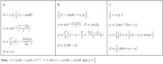
Circular sectionThe calculation formulas of geometric elements of a circular section can be deduced from formulas of a horseshoe section by replacing  (cf. Table 3).
Table 3. The calculation formulas of geometric elements of one depth zone of a circular section
 |
| |
|
3. Diameter Calculation (Governing Equations)
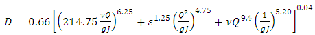
Circular section filledSwamee and Jain [17] have obtained an approximate explicit solution of the pipe diameter with a relative error of ± 2%, Rel. (3). The latter is valid for the following initial conditions: 

 | (3) |
With;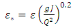 | (4) |
And,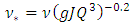 | (5) |
Where:  are respectively the flow rate, the hydraulic slope, the absolute roughness, the kinematic viscosity of the fluid and the gravitational acceleration.Thereafter, Swamee and Rathie [20] have obtained an analytical solution of the diameter, it is in form of a convergent series based on the implicit equation of Lagrange. According to these authors, the use of the expression Rel. (6) with three terms ensures sufficient accuracy and respectively two terms is sufficiently precise for all practical purposes.
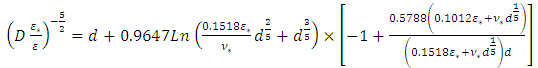 | (6) |
With;  (relations Rel. (4) and (5)) and d given by the following relationship
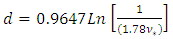 | (7) |
Furthermore, Swamee and Swamee [21] have presented the following equation Rel. (8) for the calculation of the diameter with a relative error oscillating between -2.75 and 2.75%. The error interval is valid for: 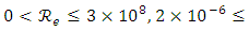

 | (8) |
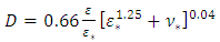
Also, Babajimopoulos and Terzidis (2013) have presented an explicit method Rel. (9) for the diameter calculation. The obtained mean relative error is of the order of 0.36%, which is valid for: 

 | (9) |
With;  (relations Rel. (4) and (5))
4. Basic Equations
By replacing the mean velocity v in the Rel. (1) by the expression  , hydraulic slope (unit head loss charge) is written as follows.
 | (10) |
Either  the geometric elements with a single depth zone Fig. (1). The hydraulic diameter
  is expressed as a function of these two parameters by the relationship below.
 | (11) |
By posing the expression  in the relationship (11), we get:
 | (12) |
With; | (13) |
By replacing Rel. (12) in (10), the hydraulic slope becomes: By replacing Rel. (12) in (10), the hydraulic slope becomes: | (14) |
With; | (15) |
 is the Reynolds number which can be expressed as follows:
 | (16) |
Subsequently, the elimination of  and
and  in the Rel. (2) is done by using the relationships (14) and (16). As a result,
  can be expressed by the following relationship.
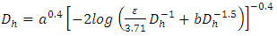 | (17) |
With; | (18) |
And; | (19) |
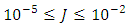
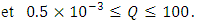
Admitting that values of ε, a and b are given, relation (17) shows that the value of the hydraulic diameter Dh cannot be explicitly determined. Indeed, the relation (17) is implicit vis-a-vis of Dh, because this one is contained in both the left and right members of the relationship. The Determining of the diameter Dh therefore requires an iterative method in the case where the relation (17) is used.Proposed RelationshipA number of 226980 exact values of  was generated by the numerical solution of the Rel. (17) with the conditions:
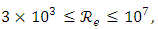
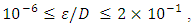
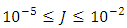 and
and 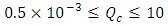 . All the necessary coefficients for the prediction of the hydraulic diameter were obtained. Firstly, by the optimization method of nonlinear equations using approximation technique, and secondly, by minimizing the maximum relative error. The relationship (20) given below predicts the hydraulic diameter
  with the desired accuracy.
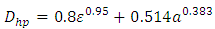 | (20) |
By introducing the relationship (20) in the second term of relationship (17), we obtain a relationship Rel. (21) expressing the estimation of hydraulic diameter Dhe.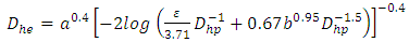 | (21) |
In order to better specify the reliability of the explicit relation (21), we have compared at that mentioned by the implied relationship (17), taken as the reference. Assuming that, for each value ε, a and b implicitly Q, J and ε are fixed and chosen in the range of application conditions, equation (17) gives, after an iterative method, an exact value and that proposed by equation (21) affects an approximate value of the hydraulic diameter.The relative errorStatistical analysis of the 226980 values estimated by the Rel. (21) and those obtained numerically by Rel. (17) shows that: a maximum relative error of the order of 0.6% and a minimum relative error of the order of  . On the basis of these two extreme errors, a calculation of the partial and cumulative frequencies is performed from the relative error orderly into ten (10) centered class. Figure 2 shows that 50% of the values obtained by Rel. (21) have lower relative errors than 0.09% and more of 80% of values have relative errors lower than 0.25%. Note that, the probability of obtaining a relative error greater than 0.45% is 3%. Furthermore, an average error of 0.17% is recorded.
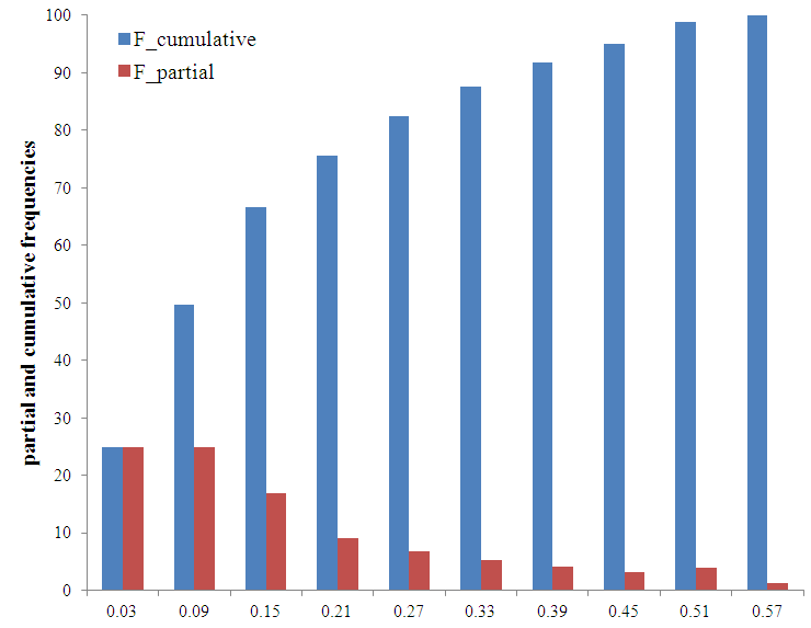 | Figure 2. Distribution of partial and of cumulative frequencies of the relative error (%) |
Figure 3 shows a perfect linear relationship between the exact hydraulic diameter calculated by the Rel. (17) and that estimated by the Rel. (21). The linear equation Fig. (3) has a coefficient of determination  that equals 0.99998 where this value judge a good linear regression between the two hydraulic diameters.
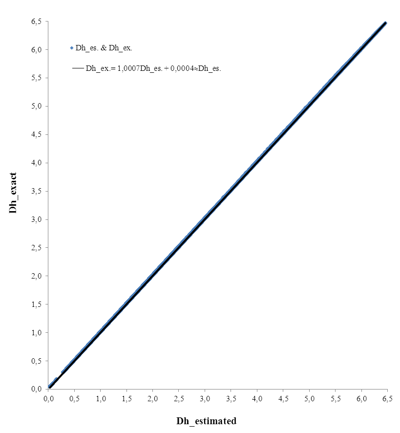 | Figure 3. Values of (Dhe) calculated by equation (21) compared to the exact values (Dh) calculated by equation (17) |
Dimensioning of a conduitNote that for a flow section of shape described by Fig. (1), the dimension  can be calculated by applying the following explicit relationship, issued from the combination of relations (11) and (21).
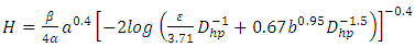 | (22) |
For the given values of the parameters  the steps of calculating of the total height H of the conduit are then as follows: The relationships (18) and (19) allow to determine the coefficients
  and
and  by replacing
  by
by  where
where  is given by relationship (13). Then,
  and
and  are introduced in the relationship (20) for predicting the hydraulic diameter
  which is than introduced in equation (22) for estimating the dimension H.Case of a circular conduit under pressureA number of 226980 exact values of the conduit diameter of circular form under pressure was calculated by solving numerically the rel. (17) by replacing
  by
by  with
with  . Application conditions obtained are:
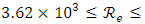


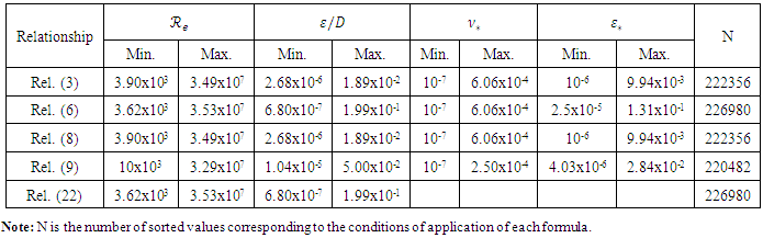
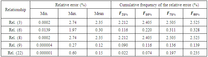
 Then, the estimated values of the diameter are calculated on basis of application conditions of each formula. The obtained results, the applications for each formula and some position parameters and their relative error dispersion are respectively summarized in the tables 4 and 5.
Table 4. Summary of the obtained results and the conditions of application of each formula
 |
| |
|
Table 5. Summary of obtained results of some position parameters and the relative error dispersion for each formula
 |
| |
|
A priori, Table 5 shows that the relationship (3) of Swamee and Jain [17] and the relation (8) of Swamee and Swamee [21] differ only in the writing of their expressions and their application conditions. In addition, the two expressions Rel. (3) and (8) gives important relative errors compared to available other formulas. The relationship (6) of Swamee and Rathie [20] is approximately eight times more precise than the two preceding. Certainly, the relationship (9) of Babajimopoulos and Terzidis [2] offers better accuracy on the maximum value, the mean and the cumulative frequency to 80%. Also, the relationship (22) "case of a circular pipe" gives a good accuracy on the minimum value and the cumulative frequency to 50%. The mean relative error obtained by the present proposed relationship is reduced of 50% comparatively than that calculated by the Rel. (6) but it is increased of 25% comparatively than that obtained by the Rel. (9).Case of a noncircular section under pressureThe conditions of the numerical experimentation are identical to those applied for a circular section. The only difference lies on the taken values of α and β. The calculation was performed, on the one hand, α = 0.5105 and β = 2.6433 for an oval section, and on the other hand, α = 0.8293 and β = 3.2669 for a section in the shape of a horseshoe. Figure 4 shows that the cumulative frequency distribution of the relative errors are almost identical between the two sections (ovoid form and horseshoe form) and the circular section. In front of this result, the dimensioning of such sections is performed at 80% of chance with a maximum relative error of the order of 0.25% and at 95% with a maximum relative error of the order of 0.40%.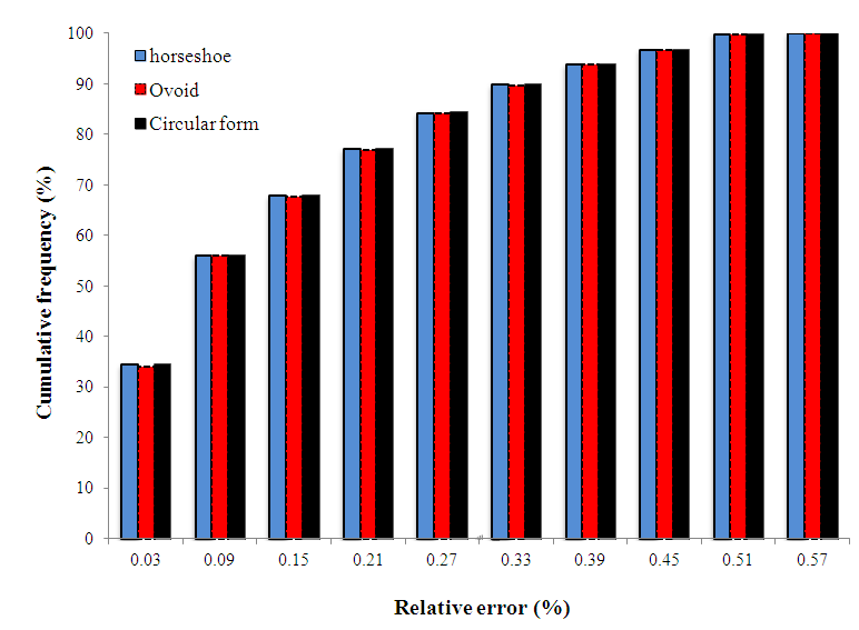 | Figure 4. Distribution of cumulative frequencies of the relative error for three cross sections of usual forms |
5. Conclusions
The relationship proposed in this paper has been applied successfully to calculate the total height that serves to dimensioning a conduit. The total height H of a conduit is an important element in the conception, the exploitation and maintenance of pipes and channels. The calculation of this element is performed either by numerical methods, graphics, and analytical approaches or by the aid of explicit regressive equations. The explicit solutions are available in the literature for the calculation of the friction coefficient λ, and consequently, for the calculation the diameter D of the pipes under pressure. The maximum relative error of the proposed relationship is less than 0.25% for 80% of calculated values and a mean relative error of 0.17%. In the case of completely filled circular conduit, the relationship is well classified among the various explicit equations mentioned in this document where it has both simplicity and accuracy. The new approach proposed in the present study offers the possibility to solve problems linked to dimensioning of pipes and channels with high accuracy comparatively to those available in the literature. Consequently, it can be used successfully for practical purposes.
List of Symbols
Q = water discharge [m3s-1]Qc = flow calculation [m3s-1]J = hydraulic gradient [m]Dh = hydraulic diameter [m]Dhp = hydraulic diameter predicts [m]Dhe = hydraulic diameter estimated [m]D = geometric diameter [m]l = length of the conduit or of the channel [m]v = mean velocity [ms-1]g = Gravitational acceleration [ms-2]Re = Reynolds number [adimensional]Ai = wetted section of rank i [m]Pi = wetted perimeter of rank i [m]hi = maximum water height of the zone of rank i [m] H = height of the conduit [m]Symbolsηi = maximum filling ratio of the zone of rank i [adimensional]ε = absolute roughness [m]η = Dimensionless [m]μ = dynamic viscosity [Nm-2s-1]ρ = density of fluid [kgm-3]θ = cross-section angle [radians]α = coefficient of the wetted section [adimensional]β = coefficient of the wetted perimeter [adimensional]τp = shear stress [Nm-2]λ = friction factor [adimensional]φ = function [adimensional]Subscripts* = [adimensional]Max = maximum value Min = minimum valuec = calculation
References
| [1] | Achour B., Bedjaoui A., Khattaoui M. and Dababeche M. (2002). “Contribution au calcul des écoulements uniformes à surface libre et en charge”. Larhyss/Journal n°1, 7-36. |
| [2] | Babajimopoulos C. and Terzidis G. (2013).”Accurate Explicit Equations for the Determination of Pipe Diameters". J. Hydraul. Eng., Vol. 2, No. 5, pp. 115-120. |
| [3] | Bedjaoui A., and Achour B. (2010). “Nouvelle approche pour le dimensionnement des conduites circulaires sous pression”. Courrier du Savoir – N°10, pp.23-29. |
| [4] | Bombardelli F., and Garcia M. (2003). "Hydraulic Design of Large-Diameter Pipes”. J. Hydraul. Eng., 129(11), 839-846. |
| [5] | Brkić D. (2011a). “New explicit correlations for turbulent flow friction factor”. Nucl. Eng. Des., 241(9), 4055-4059. |
| [6] | Colebrook C. F. (1939). “Turbulent flow in Pipes, with particular reference to the transition region between the smooth and rough pipe laws”. J. Inst. Civil Eng., 11(4), 133-156. |
| [7] | Darcy H. (1854). “Sur les recherches expérimentales relatives au mouvement des eaux dans les tuyaux”. Comptes rendus des séances de l’Académie des Sciences, Vol.38, 1109-1121. |
| [8] | Diniz V. E. M. G., and Souza P. A. (2009). “Four explicit formulae for friction factor calculation in pipe flow”. Transactions on Ecology and the Environment, 125 369-380. |
| [9] | Giustolisi O., Berardi L., and Walski T. M. (2011). “Some explicit formulations of Colebrook–White friction factor considering accuracy vs. computational speed”. Journal of Hydroinformatics, 13(3), 401-418. |
| [10] | Gulyani B. B. (2001). “Approximating equations for pipe sizing”. Chemical Engineering, 108(2), 105-108. |
| [11] | Haaland S. E. (1983). “Simple and Explicit Formulas for the Friction Factor in Turbulent Pipe Flow”. J. Fluids Eng., 105(1), 89-90. |
| [12] | Hager W.H. (1987). “Computation of turbulent conduit flows”. 3R-International, Vol.26, 116-121. |
| [13] | Imbrahim C. (2005). “Simplified equations calculates head losses in commercial pipes.” The Journal of American Science, 1(1), 1-2. |
| [14] | Jain K. (1976). “Accurate explicit equation for friction factor.” Journal of Hydraulics Division, ASCE, 102(HY5), 674-677. |
| [15] | Li P., Seem J. E. and Li Y. (2011). “A new explicit equation for accurate friction factor calculation of smooth pipes”. Int. J. Refrig., 34(6), 1535-1541. |
| [16] | Moody L. F. (1947). “An approximate formula for pipe friction factors”. Mech. Eng., 69 1005-1006. |
| [17] | Sinniger R. O. and Hager W. H. (1989). “Constructions hydrauliques”. Traité de Génie Civil, Ed. Presses Polytechniques Romandes, Vol.15, Suisse. |
| [18] | Swamee P. K. and Jain A. K. (1976). “Explicit equations for pipe flow problems”. J. Hydraul. Eng. ASCE, 102(5), 657-664. |
| [19] | Swamee P. K. and Jain A. K. (1977). “Explicit equations for pipe-flow problems”. J. Hydraulic Engineering, ASCE, 103(4), 460-463. |
| [20] | Swamee P. K. and Jain A. K. (1978). “Exact equations for pipe-flow problems”. J. Hydraulic Engineering, ASCE, 104(2), 300. |
| [21] | Swamee P. K. and Rathie P. N. (2007). “Exact equations for pipe-flow problems”. Journal of Hydraulic Research, 45(1), 131-134. |
| [22] | Swamee P. K. and Swamee N. (2007). “Full-range pipe-flow equations”. Journal of Hydraulic Research, 45(6), 841-843. |
| [23] | Valiantzas J. (2008). “Explicit Power Formula for the Darcy–Weisbach Pipe Flow Equation: Application in Optimal Pipeline Design”. J. Irrig. Drain. Eng., 134(4), 454-461. |

 Abstract
 Reference
 Full-Text PDF
 Full-text HTML