-
Paper Information
- Previous Paper
- Paper Submission
-
Journal Information
- About This Journal
- Editorial Board
- Current Issue
- Archive
- Author Guidelines
- Contact Us
International Journal of Hydraulic Engineering
p-ISSN: 2169-9771 e-ISSN: 2169-9801
2015; 4(3): 54-69
doi:10.5923/j.ijhe.20150403.02
Experimental Investigation of Influence of Vegetation on Flow Turbulence
 Abstract
 Reference
 Full-Text PDF
 Full-text HTML
Nazanin Mohammadzade Miyab1, Hossein Afzalimehr1, Vijay P. Singh2
1Department of water engineering, Isfahan University of Technology, Isfahan, Iran
2Department of Civil and Environmental Engineering, Dept. of Biological and Agricultural Engineering, Texas A&M University, USA
Correspondence to: Hossein Afzalimehr, Department of water engineering, Isfahan University of Technology, Isfahan, Iran.
| Email: |  |
Copyright © 2015 Scientific & Academic Publishing. All Rights Reserved.
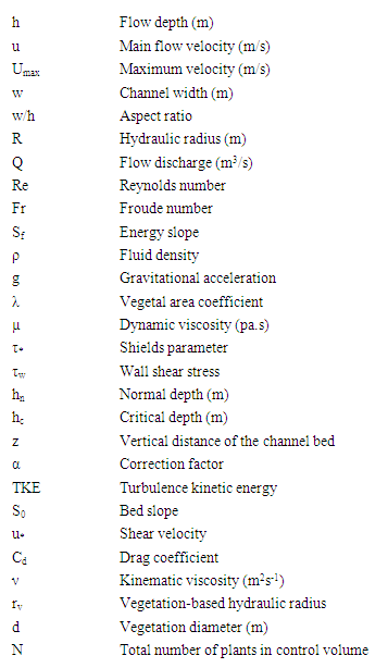
Vegetation in channels, rivers, reservoirs, and wetlands alters the flow turbulence characteristics. Vegetation has both positive and negative effects, depending on the objective of the hydraulic conduit. For example, it decreases conveyance capacity by obstructing flow by reducing the flow cross-sectional area and increasing resistance to flow and may, hence, increase flooding. On the other hand, it increases bank stability, reduces erosion and turbidity, provides habitat for aquatic and terrestrial wildlife, presents aesthetic properties, and filters pollutants. Using both field and laboratory experiments, this study investigates the influence of vegetation on turbulent characteristics and flow resistance for a channel with gravel bed and vegetation on banks. The results shows that vegetation affects the velocity distribution, the position of dip phonemenon, turbulent kinematic energy and drag coefficient. These changes can be observed in the distribution of shear stress, the quadrant analysis events and statistics moments.
Keywords: Ecosystem, Gravel bed channels, Flow resistance, Turbulence, Vegetation
Cite this paper: Nazanin Mohammadzade Miyab, Hossein Afzalimehr, Vijay P. Singh, Experimental Investigation of Influence of Vegetation on Flow Turbulence, International Journal of Hydraulic Engineering, Vol. 4 No. 3, 2015, pp. 54-69. doi: 10.5923/j.ijhe.20150403.02.
Article Outline
1. Introduction
- Vegetation growing in waterways and rivers increase turbulence. As part of ecosystems, it provides habitat for animals by creating low-flow regions [1] and improves water quality by producing oxygen and removing excess nutrients [2, 3]. It consumes a great deal of energy and current momentum along the course of rivers and floodplains [4]. Momentum transfer causes shear stress on the walls, which influences the discharge of the main channel as well as of floodplains and also the erosion and sustainability of banks and the general transfer of sediments [5].Vegetation is known to increase bank stability, reduce erosion and turbidity, provide habitat for aquatic and terrestrial wildlife, attenuate floods, present aesthetic properties, and filter pollutants [6]. Aquatic vegetation planting and management are commonly used approaches in river ecological restoration in recent years [7]. Vegetation has traditionally been viewed as an obstruction to channel flow by decreasing carrying capacity and by increasing flow resistance and the risk of flooding. In recent years, vegetation has become a major component of erosion control and stream restoration [8].The mechanism of turbulence in channels with vegetation is of considerable importance [9], especially in mountainous regions where the dominant flow regiment in rivers is turbulent flow. This is the specific feature of Iranian rivers. Flow is termed turbulent when flow characteristics are variant and the acceleration force is much stronger than the viscous force. The exclusivity of turbulence is eddy and turbulent streams exhibit 3D temporal and spatial fluctuations. For estimating surface flooding and improving flow conditions, information on flow-vegetation interaction is important. Therefore, the objective of this study is to investigate, using both laboratory and field experiments, the influence of vegetation on turbulent characteristics and flow resistance for a channel with gravel bed and vegetation on banks.
2. Methods and Materials
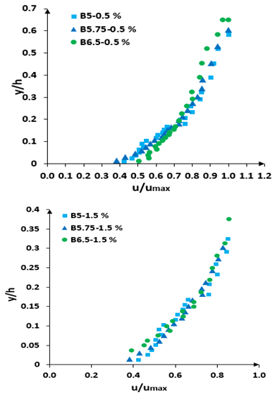
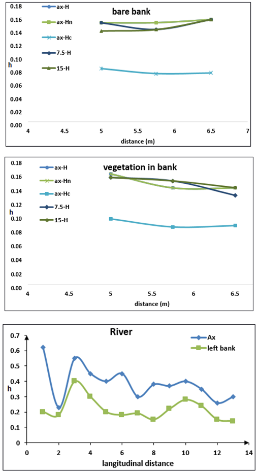
- In this study, both field and laboratory experiments were conducted. Laboratory ExperimentationFlumeAn experimental channel, located in the Hydraulics Laboratory at Isfahan University of Technology, was used for experimentation. The channel is rectangular in cross-section, 8 m long, 40 cm wide, and 60 cm deep. The channel wall and floor are made up of clear Plexiglas. The flow discharge and depth used were equal to 40 liters/s and an average of 15 cm, respectively.Laboratory Experiments Experiments were conducted in 4 series, including 2 series with and without vegetation in which the bed slope was chosen as 0.5%, and 2 series with and without vegetation with a bed slope of 1.5%. A total of 40 velocity profiles were measured. For each profile, the point velocity was also calculated at 20-25 points along the depth of flow.In order to keep measurements in order, it was found appropriate to use the following nomenclature. If there was vegetation then letter R (Rice) and if there was no vegetation then letter B (Bare bank) were used at the beginning of the profile and then were used the distance from the central axis in centimeter and the distance from the beginning of the channel in meter and the slope of the channel bed, respectively. For example, B0-6.5-0.5% indicates bare bank with a slope of 0.5% and the distance of 6.5 meters from the beginning of channel in central axis.To investigate the development of flow, the fourth series of experiments measured profiles in the central axis that had 5, 5.75 and 6.5 m distance from the beginning of channel, as shown in figure 1. The figure 1 shows that the distance of 5 m from the entrance of the channel is suitable to verify the fully developed flow condition where the velocity distributions are auto-similar.
 | Figure 1. Development of flow in channel |
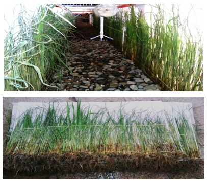 | Figure 2. Gravel bed and vegetation in bank |
|
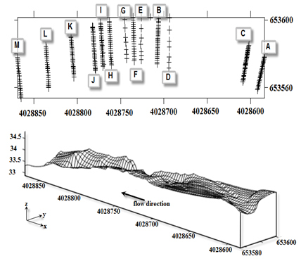 | Figure 3. Topography and post-maps display of the study reach |
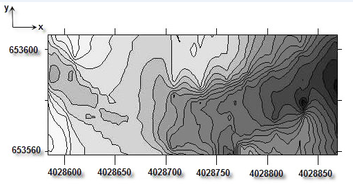 | Figure 4. Display contour line of selected reach |
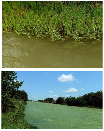 | Figure 5. Display of vegetation in banks in selected reach of Babolrod River |
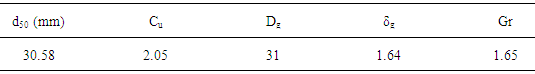
 Cu = 2.05 which is suggestive of the particle uniformity. Also, the average geometric measure Dg, geometric scale deviancy δg and gravel coefficient Gr were included, as shown in table 2.
|
|
 | (1) |
 | (2) |
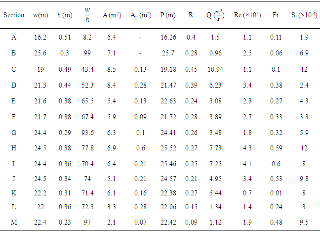
 , R is the hydraulic radius (m), µ is the dynamic viscosity (Pa.s), h is the water depth (m), and g is the gravitational acceleration.According to table 3 in the field case, since the Reynolds number was 2×10⁵ the flow was unsteady and Froude number was 0.3 which indicated subcritical flow.The Reynolds number was from 12.5×10⁵ to 6×10⁴ for the laboratory experiments. This indicated that the flow regime can be considered as turbulent flow. The flow was subcritical because the Froude number was less than 1 for all laboratory experiments.Colosimu et al. [10] and Afzalimehr and Anctil [11] introduced the Shields parameter as one of the parameters influencing the flow resistance in uniform flow. This dimensionless parameter can be defined as follows:
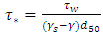 | (3) |
 | (4) |
 | (5) |
 | (6) |
 | (7) |
 and
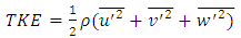
and  are the fluctuations of u, v and w, respectively [10].The turbulence kinetic energy is an important hydraulic parameter to evaluate the turbulent structure [13]. Turbulence in open channel flow may significantly affect the localized erosion in channel [12]. Actually, the effect of vegetation on turbulent structure depends on multifaceted and interacting factors [14]. Because of the tedious experimental procedures [15], TKE is difficult to experimentally determine.Shear velocity is one of the factors that directly affect the calculation of resistance coefficient. Thus, the method applied for the calculation is important. This value was estimated by different methods, such as log law (Clauser method), parabolic law, Saint-Venant equation, boundary layer theory, energy gradients, and Reynolds shear stress. In this research, the Saint-Venant equation was used as follows:
 | (8) |
 | (9) |
 | (10) |
 | (11) |
 | (12) |
 | (13) |
 | (14) |
3. Results and Discussion
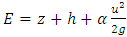
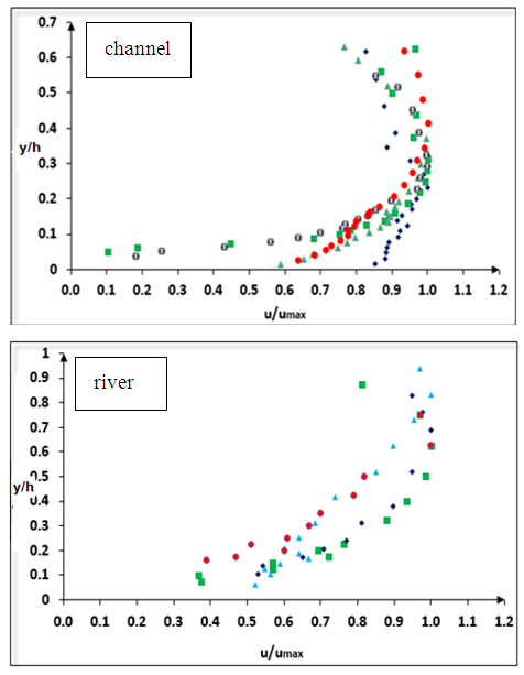
- Effects of vegetation on flow velocity distribution Flow velocity is an important parameter for evaluating the flow field structure in an open channel flow, especially for non-scouring and non-silting velocities, which affects the soil erosion in rivers [25]. The secondary current can affect the flow structure and change the position of maximum velocity (Umax). Figure 6 shows the velocity distribution for channel and field data, showing that Umax occurs under the water surface with and without vegetation on the bank.
 | Figure 6. Distribution of flow velocity |
 | Figure 7. Water surface in field and experimental condition |
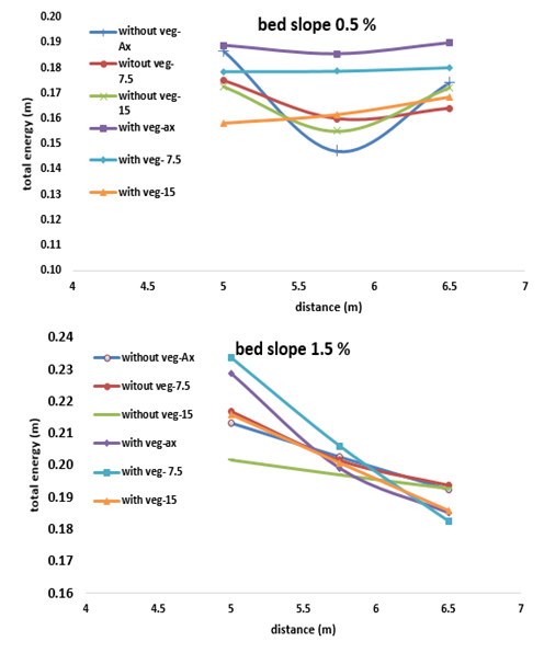 | Figure 8. Variation of total energy in experimental case |
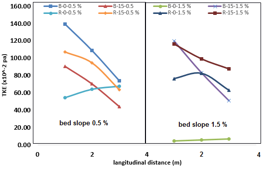 | Figure 9. The TKE values along the measured sections |
 . The results of the study made on the distribution of dimensionless shear stress, with and without vegetation, are as follows:1) For the bare bank condition, 18 profiles were studied. In 15 profiles, the amount of shear stress in
  first increased and then from
  showed a decrease. The range of alterations of
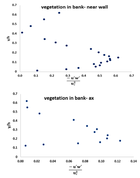
  was between 0.07 and 0.3. In the 3 profiles left, the change in the shear stress was of a decreasing line. The maximum of shear stress was observed near the bed in all these profiles.2) For the condition of existing vegetation, in 17 cases, the profiles of the distribution of shear stress were in 3 parts: Part 1: an increase of Reynolds stress near the bed
 , part 2: a decrease in Reynolds stress
 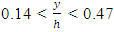 , and part 3: when
  in which the Reynolds shear increased once more. Only in one profile, there was first an increase and then a decrease.3) With the existence of vegetation, the turning point of the curve moved down and approached the bed. The creation of part 3 of the profiles was also because of the existence of vegetation. It is a bit difficult to realize whether or not there would be part 3 in profiles without vegetation, since the device ADV had some limitations measuring the point 5 cm away from the water surface.4) Comparing the central axis profiles at -7.5 cm and 5 cm from the wall, we can conclude that the less distance from the vegetation, the more negative figures will appear because of being near the vegetation and the increase in the shear stress level of the momentum absorption. Also the maximum shear stress occurs near the bed.
 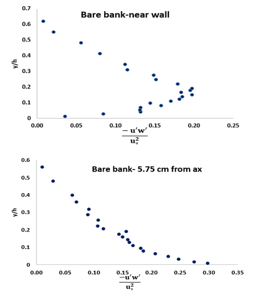 | Figure 10. Distribution of shear stress without vegetation |
 | Figure 11. Distribution of shear stress with vegetation |
 . When there was vegetation, one could observe 3 parts for distributing the velocity turbulence; and the distribution was in accordance with the Reynolds shear stress exactly. The profiles near the central axes displayed more intense curve than that of the walls. Figure 12 shows the sample distribution of RMS (u, v, w).
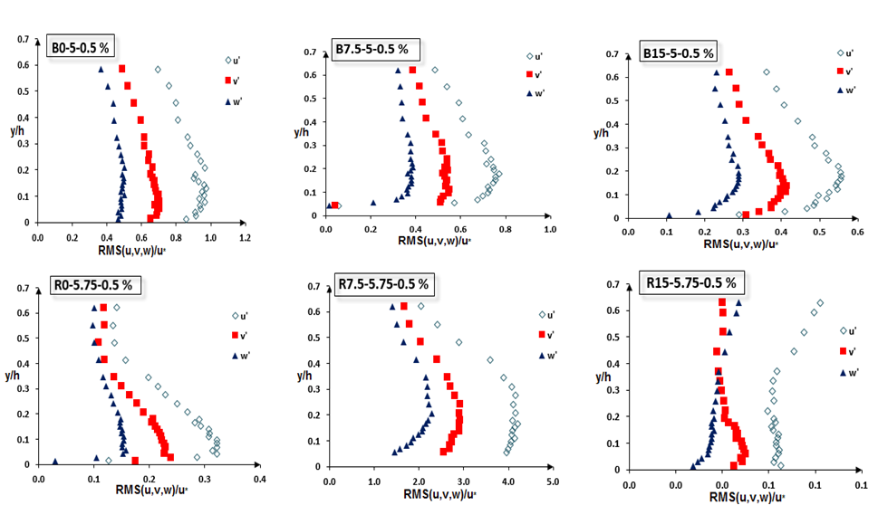 | Figure 12. Sample distribution of RMS (u,v,w) |
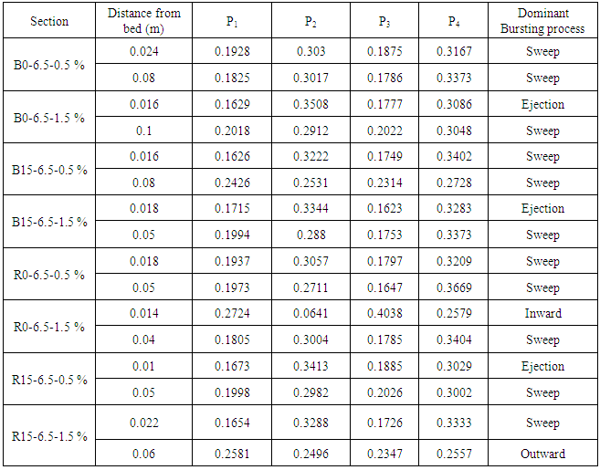
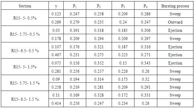
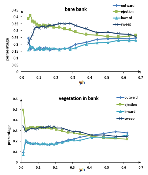 | Figure 13. Dominant turbulent events over the entire flow depth |
 , and the second region with a water depth of
  . In the first region, the variation of frequent events (ejection and sweep) was intense. In this region, ejection and then sweep were the most frequent events, while the outward and inward events had small contributions. In the second region, the variation of contribution was little and the dominant event was sweep and the contribution of outward and inward events increased. It means that events there had a significant role in the region near the water surface. Also, this plot had two regions for condition that had vegetation on bank.The first region with a water depth
  , and the second region with a water depth
  . In the first region the dominant event was ejection, followed by sweep, then inward and outward interaction, respectively. In the second region, the contribution of outward and inward interaction increased.Thus, it can be concluded that in both conditions of with and without vegetation on bank, whenever we got closer to the water surface the distribution of outward and inward interaction increased. It was intensified by vegetation due to the production of turbulence. In agreement with Fazel (2014), it seems that turbulence was much less anisotropic near the vegetated wall compared to that along the center of flume, showing contributions in all four quadrants [16].Figure 14 shows the contribution of each quadrant to the stress fraction. Similar to figure 13, the plot of y/h against the stress fraction can be divided into two regions. In the bare bank condition, ejection and sweep events had the highest distribution, but closer to water surface the distribution of their events decreased. In the condition with vegetation compared to bare bank condition, in the second region the distributions of outward and inward events were more than sweep and ejection.
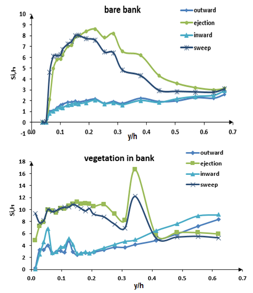 | Figure 14. Contribution of each quadrant to the stress fraction |
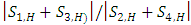 , where S2,H and S4,H are negative, called the exuberance ratio (ER). This ratio is a measurement of the upward momentum transfer against the overall downward flux, showing the exuberant nature of flow. This ratio increases in both cases (with and without vegetation on the bank) from the channel bed towards the water surface.
 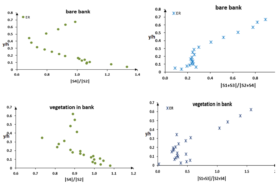 | Figure 15. The ratio of upward and downward components |
|
|
 | Figure 16. Statistics moments in the direction of Z |
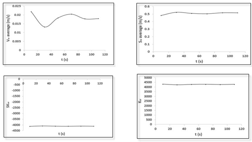 | Figure 17. Statistics moments in the direction of Z |
 were drawn as shown in figure 18.
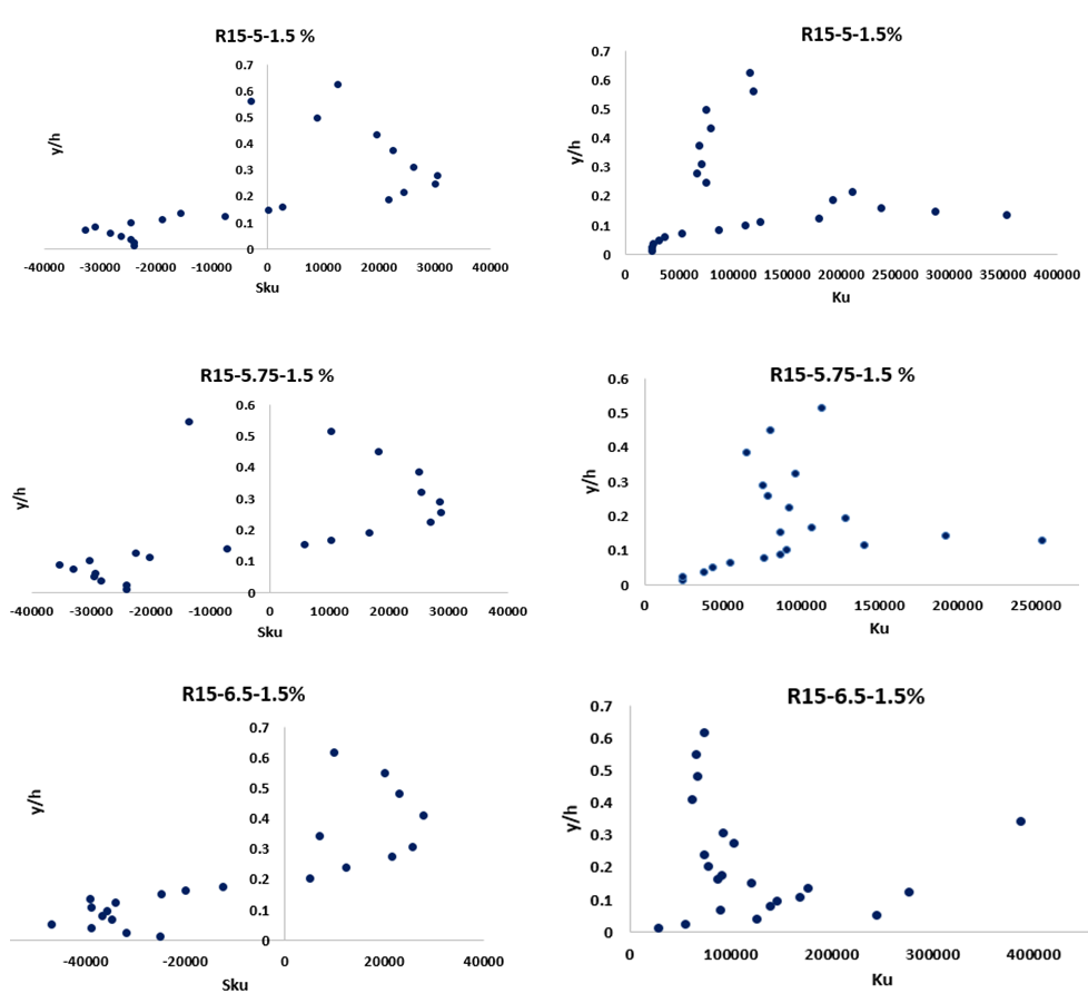 | Figure 18. A sample of the 3rd and 4th statistical moment with vegetation in spatially–based form |
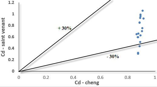 | Figure 19. Comparison of Drag Coefficient Calculated by Equations 7 and 10 |
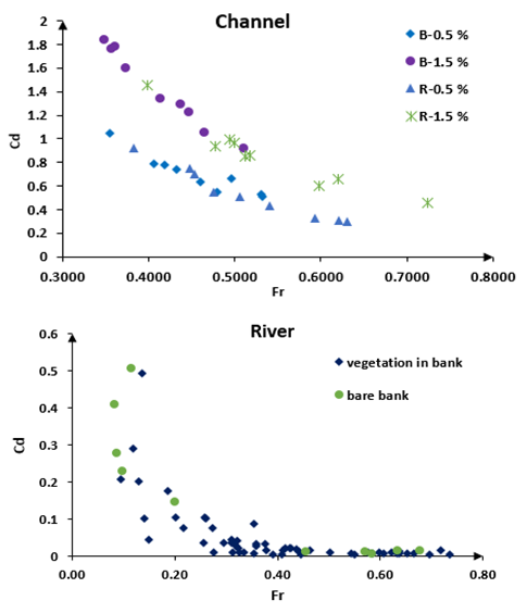 | Figure 20. The relation between Froude number and Cd |
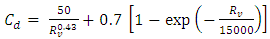
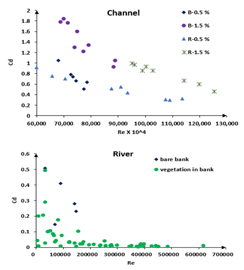 | Figure 21. The relation between Reynolds number and Cd |
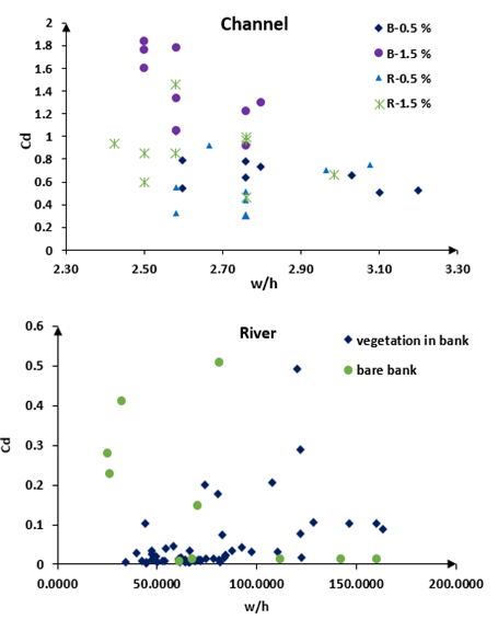 | Figure 22. The relation between aspect ratio and Cd |
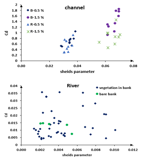 | Figure 23. The relation between Cd and shields parameter |
4. Conclusions
- The following conclusions are drawn from this study:(1) Umax occurs under the water surface with and without vegetation on the bank. It occurs under water surface for 47 and 34 percent of all measured profiles, respectively, under flow conditions of channel with w/h = 2.7 and field experiments with w/h = 80.(2) Under the condition of vegetation on banks and gradually varied flow, the dip phenomenon occurred at 65% of the water depth. It was at 50% of flow depth for bare banks and at 29% of flow depth for field data. (3) The total kinetic energy (TKE) values were more for banks with vegetation than for bare banks. The lower TKE values belong to the center axis of channel and the higher values are for near wall. (4) For vegetation, the distribution of shear stress contained 3 parts: Part 1: an increase of Reynolds stress near the bed
 , part 2: a decrease in Reynolds stress
  , and part 3: when
  in which the Reynolds shear increased once more. (5) Turbulence was much less anisotropic near the vegetated wall compared to that along the center of flume.(6) Vegetation reduced the variation of drag coefficient. (7) For laboratory experiments, the relation between Cd and Fr was an exponential decline. Vegetation and an increase in bed slope increased the variation of Cd. For field experiments, for Fr>0.45 the variation of Cd inclined towards a constant amount.(8) Drag coefficient (Cd) for small aspect ratio (laboratory run) is greater than large aspect ratios (field runs). Also, there is a direct relation between Cd and Shields parameter for small aspect ratios, while no relation was observed for large aspect ratios.
Notation