-
Paper Information
- Paper Submission
-
Journal Information
- About This Journal
- Editorial Board
- Current Issue
- Archive
- Author Guidelines
- Contact Us
International Journal of Hydraulic Engineering
p-ISSN: 2169-9771 e-ISSN: 2169-9801
2015; 4(2): 37-44
doi:10.5923/j.ijhe.20150402.03
Optimization of the Designed Water Distribution System Using MATLAB
 Abstract
 Reference
 Full-Text PDF
 Full-text HTML
Al-Amin D. Bello1, Waheed A. Alayande2, Johnson A. Otun3, Abubakar Ismail3, Umar F. Lawan1
1Faculty of Civil Engineering, Universiti Teknologi Malaysia, Johor Bahru, Malaysia
2National Water Resources Institute (NWRI) Mando, Kaduna State, Nigeria
3Department of Water Resources and Environmental Engineering, Ahmadu Bello University Zaria, Nigeria
Correspondence to: Al-Amin D. Bello, Faculty of Civil Engineering, Universiti Teknologi Malaysia, Johor Bahru, Malaysia.
| Email: |  |
Copyright © 2015 Scientific & Academic Publishing. All Rights Reserved.
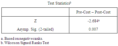
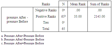
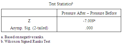
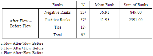
This paper provides a technique of cost optimization for the proposed water distribution system before implementation. A lot of existing water distribution network analysis software lack optimization modules but ensure other essential conditions are satisfied. Dukku Town chose as a case study, it suffers from poor water distribution network which called for the system upgrade. The models developed by Alperovits and Shamir (1977) and modified by Goulter and Coal (1986) were used to accomplish the desire objectives. A programme is written in MATLAB using linear optimization components to compute the least cost possible. Changes in pipe diameters were obtained and there is slight significant decrease in total cost of pipes. A total of 7.15% reductions in the initial cost are noted, as the hydraulic properties of the entire distribution network is improved. The maximum pressure before optimization is 14.79m and after optimization increased to 15.71m, the minimum pressure on the former is 7.59m and 9.42m for the later. The same improvement is observed in the flow rate, velocities and Headloss, all falls within the designed criterion. The efficiency of the network and risk is also considered by incorporating reliability constraint. The final optimized designed water distribution network addresses the problem of the water shortage of the studied area.
Keywords: Optimization, Linear programming, MATLAB, Statistical Analysis, Dukku town
Cite this paper: Al-Amin D. Bello, Waheed A. Alayande, Johnson A. Otun, Abubakar Ismail, Umar F. Lawan, Optimization of the Designed Water Distribution System Using MATLAB, International Journal of Hydraulic Engineering, Vol. 4 No. 2, 2015, pp. 37-44. doi: 10.5923/j.ijhe.20150402.03.
Article Outline
1. Introduction
- A water distribution system (WDS) is a hydraulic conveyance system laid on road shoulders where topology and topography are known and that transmit water from the Source to the consumers; it consists of elements such as pipes, valves, pumps, tanks and reservoirs, flow regulating and control devices [1]. Water supply system efficiency is of primary importance in designing either new water distribution networks or expanding existing ones [2]. A WDS is normally designed and operated to satisfy various customer demands over its service life. Decision makers always explore innovative and efficient strategies to reduce the huge economic requirements of designing and construction of WDS, coupled with satisfying the quantity and performance objective of the system [3]. With significant development of urbanized areas and construction of thousands of small and large-scale water supply and distribution systems in recent decades, yet few people have access to clean water and adequate sanitation. However the quality of service provided by water utilities are unsatisfactorily and the cost of new systems are expensive [4]. In order to provide a reliable framework for system’s operation, it is necessary to identify the most critical system requirement with a least cost that will enhance proper deliverance and effective operational management [5]. A lot of Research had been conducted to achieve these objectives [6-12]. Although pipe sizes and cost are the most important components of a water supply networks but other element are also considered because any water distribution network consists of three major parts and components: namely pumps, distribution storages, and distribution piping network [13]. Although in optimizing a system, the designer must take some expected and unexpected loading conditions into consideration to ensure effective and sufficient deliverance of water to end user [14]. Selection of pipe diameters from a set of commercially available diameters to form a water distribution network of least capital cost has been shown to be a difficult task [1]. The cost of maintenance and operation of a water distribution system may be considerable, but still one of the main costs is that of the pipelines. The use of optimization methods for WDS has been mostly discussed over the last decades. Optimizing WDS involves the resolution of two issues: such as design and operations [14]. Design optimization usually deals with pipes sizes while WDS operation optimization takes into account of the pump schedules [15]. In recent years a number of optimization techniques have been developed mainly for the cost minimization aspect of network planning, although some reliability studies and stochastic modelling of demands have been attempted [1]. Some of the earlier studies utilized linear programming [16-18], while later studies applied nonlinear programming (NP) [19-21] or chance constrained [20] to the pipe network optimization problem. Much of the recent literature has utilized genetic algorithms for the determination of low cost water distribution network design and they have been shown to have several advantages over more traditional optimization methods [22, 23]. Linear optimization methods have been widely studied for the case of determining optimal design of water distribution networks [24, 25].
2. Material and Methods
2.1. Description of the Study Area
- Dukku is the headquarter of Dukku Local Government Area (LGA) of Gombe State (Fig. 1). The LGA has an Area of 3,815km2 and Population of 207,190 as at 2006 census. Dukku is located at Latitude 10.82° N and Longitude 10.77° E with Elevation of 608 m above sea level.
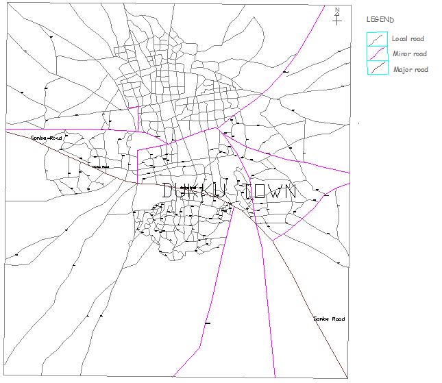 | Figure 1. Dukku town |
2.2. Dukku Water Supply System
- The Dukku water supply source is purely underground water source and the town draws its water supply from a network of five boreholes drilled on the floodplains of the River Abba along the Gombe – Darazo road. The first three sets of borehole were drilled in 1975 and two additional one were drilled by the Upper Benue River Basin Development Authority. Average water discharge from the boreholes is about 320m3/hr.The boreholes discharge water through a 15km long 300mm diameter ductile iron rising mains to the booster station near Wuro-Tara. The booster pumps also pump through another 15km rising mains 250mm ductile iron pipe to deliver water to Dukku. The initial design of WDS layout before optimization is shown in figure 2.
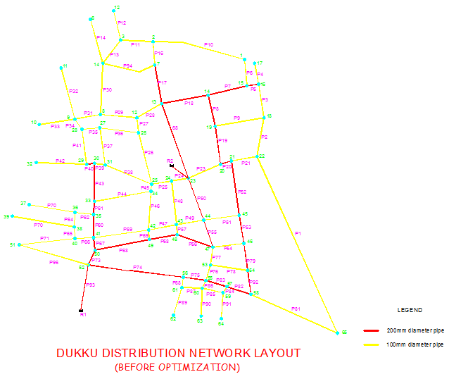 | Figure 2. WDN Layout before optimization [26] |
2.3. Software and Programming Tool Used
- Water Distribution Network optimization analysis have broad components and complexity in terms of analysis and problem solving [27]. Therefore, a lot of programmes are developed to solved those problems and it required flexible, simple to write and easier to understand concepts. For this study MATLAB (matrix laboratory) developed by MathWork [28]
 because it can solve many technical computational problems, especially those with matrix and vector formulations, in a fraction of the time it would take to write a program in a scalar non-interactive language as compared to C or FORTRAN [29]. EPANET water distribution network analysis software is employed to analyze the network. This solver uses the basic hydraulic principles to solve and analyze WDN [30], of which the results obtained in the solver are prepared as an input file for MATLAB to Optimized.
2.4. Optimization Procedure
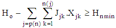
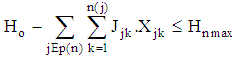
- This approach, which seeks to determine the pipe sizes and associated lengths so as to minimize the cost of the system while satisfying hydraulic criteria and reliability requirements, is derived from a model developed by Goulter and Coals [31] which in turn is originated from an earlier model developed by Alperovits and Shamir [16] with slight modification, as shown below.Objective Function:Minimization of network CostThe objective function used to minimize the network cost for the Dukku water supply system formulated as [16, 29] given in equation 1
 | (1) |
 | (2) |
 | (3) |
 | (4) |
 | (5) |
 | (6) |
 | (7) |
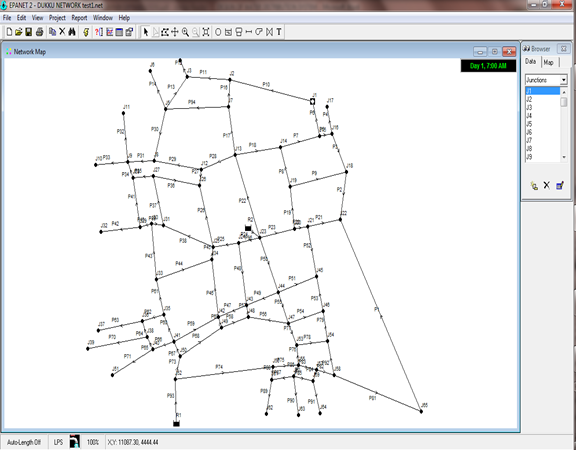 | Figure 3. Showing Dukku Network in EPANET Interface |
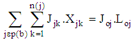
 And, Ho-Hmin = H, Hmax-Ho=HLWhere;H0 = Head of the Reservoir (m)Hmax = Maximum allowable head (m) in the Network-User defineHmin = Minimum allowable head (m) in the Network-User defineH1, h2, h3, h4 = Are the respective unit head loss of the sample diameter of corresponding lengths X1, X2, X3, X4 (Determine by LOP using Hazen William Equation) in the Programme the H and HL are User-defineConstraints 3: It is also called Equality constraint in LOP programme, as shown in Equation (5.0)Is converted as; X1h1+X2h2+X3h3+X4h4 = LoHWhere;L = total length of the link in viewH = Head loss generated by the EPANET corresponding to the link in viewConstraints 4: LOP defines it as Bound constraints, Equation (6.0). This constraint makes all the variables in the forms
 Constraints 5: LOP defines it as a Matrix of define Rows and Column and its called Inequality Constraints, Equation (7.0)It is converted to matrix form in this format
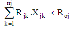
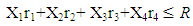 Where;R = it is the expected number of break (greater than or equal to zero) per year in the whole network (user define)r1,r2,r3,r4 = the expected number of breaks per km per year corresponding to the variables X1,X2,X3,X4.The program is run, and the output result is display in a text formatStep 6, 7, 8 and 9 of algorithm: output the result obtained in MATLAB codeAfter the result is obtained in the text format, the respective diameters of each link is observed and the diameter with higher length is chosen or if the length is relatively close to the higher length but shifted significantly on the diameter that is higher than the initial diameter, the observed changes are then updated and the solver is re-run again. The result obtained in the solver is compare to the previous result and if all condition are satisfied then optimization done. The Condition includesi. Are the design condition satisfiedii. Is the flow direction constantThese procedures are maintained for all the links and updated in the Solver until all the conditions are satisfied.
3. Result and Discussion
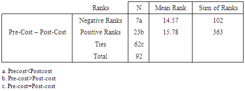
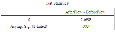
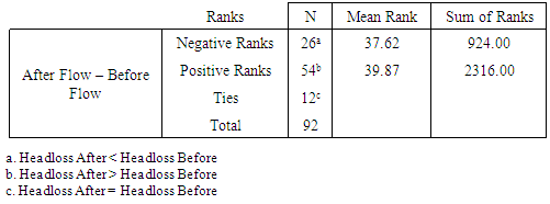
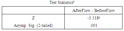
- The result shows additional 150mm and 250mm size pipes in the network. The network in the end has four different sizes of pipes (Water Distribution Network layout of the study area is updated as shown in fig. 3) unlike the initial designed that considered two different sizes, 100mm and 200mm only (fig. 2).In other to ascertain the significant of the optimization, a statistical analysis was used and the results obtained are explained according to the desired parameters and importance.
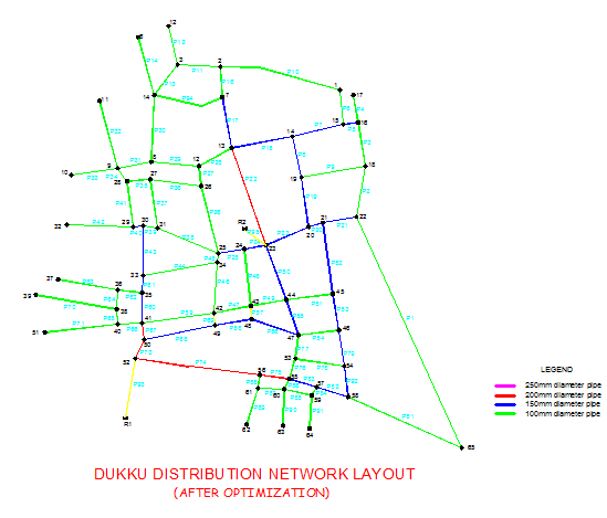 | Figure 4. WDN layout after Optimization |
|
|
|
|
|
|
|
|
4. Conclusions
- Both the capital and maintenance cost of a water distribution network (not including operation cost) is enormous. As a result design Engineers are looking for new approach for the best design of water distribution networks in addition with the usual methods. In this research, a methodology is designed which uses an optimization procedure employing linear relationship of the model parameters (LOP) while the objective function ensured minimization of the capital cost of the pipes. A designed Network of Dukku water distribution system is used as a case study. Instead of using an Extended period simulation (EPS) in running the solver, a single period simulation (SPS) is used due to the sources of the water which was mainly Bore hole.Although the WDS is initially design with two types of pipes (200mm and 100mm pipes), and being that the minimum acceptable pipe size for any WDS is 100mm, the optimization is done using pipes of 100mm,150mm, 200mm and 250mm diameters. There is a total decreased of 7.15% (direct comparison) of the initial estimate of the pipes. But using statistical comparison it shows slight (minimal) significant differences of the cost before and after optimization. In terms of hydraulic properties the network is more efficient and pressures can accommodate peak demand at every part of the distribution network which solves the problems of water shortage in Dukku if implemented.It is important to know that a node isolation approach can be used especially in the decision making process for improving the network if a limited amount of money is available.
ACKNOWLEDGEMENTS
- This study is supported by Spicks Associates a Water Resources based Consultants. The authors wish to acknowledge the help and corporation received from the staff of the Water Resources and Environmental Engineering (ABU) Zaria in conducting this research work, and all other relevant agencies that make the research possible.