1. Introduction

Vegetation in natural channels and river flood plains influences the flow field and related phenomena, like erosion and sedimentation, nutrients, pollutant and metal transport, wave energy dissipation, and life of microorganisms ([1-7]).

The study of flow and turbulence characteristics in vegetated open channels has been of great interest over the past couple of decades. For studying the flow above and within the vegetation both experimental and numerical approaches have been used [8].

Vegetation is flexible in varying degrees, and it oscillates in the flow, changing position. In vegetated channels, flow depth and the nature of vegetation as hydraulic roughness may vary widely. The depth of flow may be such that it is less than or equal to (large-scale roughness), or greater than (small-scale roughness) vegetation height. Flow in a vegetated channel is essentially a movable boundary problem, since roughness elements are deformed by the flow within the channel [9]. Two types of vegetation are usually defined: stiff and flexible. Flexible herbaceous vegetation is widely used as a protective liner in agricultural waterways, flood channels and emergency spillways [10].

According to Gourley (1970) there are three layers in the experimental velocity profiles in a vegetated bed channel: (1) a layer of virtually constant low velocity within the grass near the bed in which the velocity can be assumed proportional to the shear velocity; (2) a layer of rapidly increasing velocity within the upper part of the vegetation elements; (3) a layer of less rapidly increasing velocity above the grass [11]. Kouwen et al. (1969) distinguished a logarithm velocity profile over artificial flexible vegetation (strips of styrene) [12].

Based on experimental studies of Carollo et al. (2002) all the measured velocity distributions were S-shaped, as observed by previous studies on flow in vegetated channels. For each experimental profile three zones were identified: zone Ι inside the vegetation, characterized by very small velocities; zone ΙΙ in which the logarithm velocity can be fitted to the measured velocities (logarithm zone); and zone ΙΙΙ characterized by positive vertical velocity gradients, progressively decreasing to zero near the free surface where the velocity profile becomes vertical (free stream zone) [9]. In addition to affecting the mean velocity, vegetation also affects the turbulence intensity and the Reynolds stress [13]. Jarvela (2005) showed that the flow structure above the submerged young wheat was comparable to that found in the studies involving flexible vegetation. The flow above the wheat reasonably followed the log law and maximum values of u_rms and -u'w' were found approximately at deflected plant height. The velocity profile showed an inflection point which superposes with the maximum turbulence and it occurs above the vegetation cover [10]. Also the Reynolds stress distribution revealed its maximum value above the upper limit of the vegetation cover [14].

In previous works over vegetated beds, researchers have not considered the non-uniformity of flow. In nature, due to the topography of bed, most of the time, the flow is not uniform, therefore the study of non-uniformity of flow over vegetated beds is essential to understand the hydraulic parameters distributions. In this study, the case of unfavorable pressure gradient (decelerating flow) over the vegetated bed in a laboratory flume is investigated. The aim of the study is to determine how the interaction of vegetation bed and pressure gradient affects the main flow velocity, turbulence and Reynolds stress distributions. Also, the validity of the log law in the inner layer and Coles method in the outer layer are investigated.

2. Experimental Setup and Measurements

Experiments were conducted in a 8-m long, 0.4-m wide and 0.6-m deep flume with plexiglas walls in the hydraulics laboratory of Isfahan University of Technology, Iran. To produce a decelerating flow where the pressure gradient is adverse, gravel with different heights from the flume bed were deposited in the flume. Then, grass seeds, which were cultivated in metal boxes 0.4-m long, 0.2-m wide and 0.05-m deep, were transferred to the laboratory and were placed over the gravel in the flume. The entire length of the flume bed was covered with grass. We tried to keep the height of the grass constant (about 8-cm) during measurements. The density of the grass was 27000 stems per square meter.

A movable downstream weir was used to change the depth of flow. An upstream storage reservoir was used to reduce the flow entrance turbulence. Our experiments were conducted in four runs with two different depths of flow (0.15m and 0.2 m at section 6-m from the entrance of the flume) and two different flow discharges (5.7 l/s and 7.2 l/s). The slope of the flume bed was set as 2%. The slope of the bed was formed by using gravel along the flume.

Velocity measurements were performed by using an Acoustic Doppler Velocimeter (ADV). The ADV is a 200-Hz Nortek Vectrino. To remove possible aliasing effects, the velocity time series were analyzed using WinADV [15], which is a windows based viewing and post-processing utility for ADV files. This software provides signal quality information in the form of a correlation coefficient (COR) and signal to noise ratio (SNR). Almost 75% data were considered suitable using WinADV criteria Correlation coefficient >90% and signal to noise ratio (SNR) >20. The data of the poor quality were removed from this study and were not replaced. At each point, the flow velocity was sampled with a frequency of 200-Hz and 120 seconds (our last experiences revealed that this duration for sampling is adequate for determining accurate turbulence statistics).

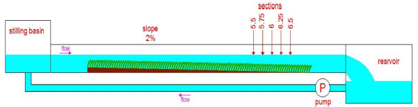Figure 1. Schematic picture of experimental setup

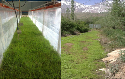Figure 2. Comparison between the experimental setup and a natural channel

Velocity measurements were made along five cross sections at x=5.5m, x=5.75m, x=6m, x=6.25m and x=6.5m downstream of the flume entrance. At each cross section, velocity measurements were made at different transverse-wise distances from the flume wall (D=5cm, 10cm, 15cm and 20cm). For each velocity profile, measurements were done from the surface of water to the canopy region. The measurements near the canopy region were conducted with lesser distances to show the velocity components changes in shear layer with higher precision.

3. Experimental Results and Discussion

3.1. Velocity Distribution

Based on velocity profiles in Fig.3, three regions can be distinguished: (1) the region where the flow is at the top of canopy; in this region ADV is able to collect data. In this region, however, the values of velocity have low gradient; (2) the region where an inflection point exists, showing the contribution of unfavorable pressure gradient in the flow velocity distribution. In this region the velocity gradient and the shear stress are considerable; and (3) the region near the water surface where velocity profile tends to approach a vertical lineshowing low shear stress and the maximum flow velocity.

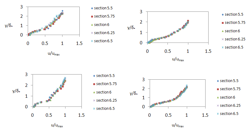Figure 3. Measured velocity profiles for all test series

The velocity distribution can be divided into two layers; inner layer where the effect of vegetation roughness is dominant and the outer layer where the maximum velocity and the boundary layer as well as the pressure gradient effect are among the controlling parameters of flow.

The velocity distribution over different artificial and natural roughness may be represented by the logarithm law:

(1)

Where, u = the mean point velocity, u_*=the shear velocity, y = the vertical coordinate, κ = the von Karman constant which is taken 0.4, K_s = roughness scale and C = a constant.

Kummu (2002) pointed out that the vertical velocity profile above vegetation bed has the logarithmic distribution only in the middle part of the profile [16]. However, Fig.4 shows that for a non-uniform flow with unfavorable pressure gradient the log law is valid near the vegetation cover. As reported by Nezu and Rodi (1986), when the distance from the bed increases, the log-law is not more valid (Fig.4) showing that the log law is applied in the inner layer and data deviate from this layer in the outer layer [17]. Many researchers have shown that the log law velocity is universal, however, the thickness of where this law is valid depends on the flow conditions and boundary conditions. In the outer layer where the velocity data do not follow the log law, no universal law exists, requiring empirical methods to explain the fitness of data in this region. One of experimental methods is the law of defect velocity. This law has shown very interesting fitness to flow over gravel bed streams under different pressure gradients [18]. The existence of stress in the outer layer results in drag on the flow and produces a velocity defect (u_max - u). The dimensional analysis reveals that (u_max - u)/ u_* can be represented as a function of y/δ where δ is the thickness of boundary layer, y is the distance from the vegetation crest and u_* is the shear velocity. Fig.5 shows that the defect velocity fits reasonably well in the outer layer region for flow over the vegetated bed under unfavorable pressure gradient flow.

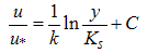
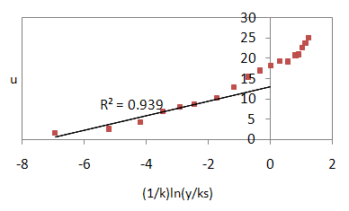Figure 4. Logarithm law validity in the inner layer

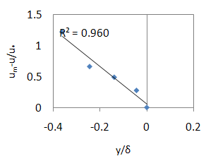Figure 5. Defect velocity validity in the outer layer

Table.1 presents a summary of measured and computed parameters in this study.

Table 1. A summary of the measured and computed data

Fig.6 shows velocity profiles along the flume. Unfavorable pressure gradient and Helmholtz-Kelvin instability cause the point velocities to tend to decrease as the flow moves downstream, showing a clear inflection point near the vegetation cover for each velocity distribution. The larger unfavorable pressure gradient is, the higher the location of inflection point is.

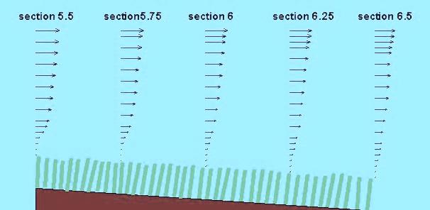Figure 6. Change of velocity profiles along the flume

Here δ_*=displacement thickness of boundary layer, θ=momentum thickness of boundary layer and β=pressure gradient parameter are defined as follows:

(2)

(3)

(4)

According to Graf (1998), parameters δ_* and θ increase along the flume for a decelerating flow in a channel with gravel bed [18]. As can be seen from Table 1, these parameters increase for the vegetated bed under unfavorable pressure gradient flow.

To quantify non-uniform flow, Graf (1998) presented a parameter (β) in which the values of β should be greater than -1 for unfavorable pressure gradient flow [18]. This criterion is confirmed over vegetated bed as well (Table 1).

The shear velocity (u_*) was calculated by using the boundary layer characteristics method [19]. The flow was subcritical (Fr<1) during all experiments.

3.2. Reynolds Stress and Turbulence Intensity

In turbulent flows, due to rapid fluctuations of velocity components, there is momentum transfer between the layers of flow. The main factors that have to be taken into account in turbulent flow studies are Reynolds stress and turbulence intensity. The main component of Reynolds stress τ_xy is represented by:

(5)

The root mean square of the main velocity component (u_rms) is defined as follows:

(6)

The velocity fluctuations were measured by ADV in x, y and z directions. Fig.7 shows the distribution of u'v' where u' and v' are velocity fluctuations in the main and vertical flow directions. Several studies have reported that the maximum turbulence intensity is found at the top level of vegetation [20, 21]. In the present study, it is observed from Fig.7 and 8 that the maximum Reynolds stress and turbulence intensity also occur at the top of vegetation.

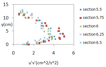Figure 7. Reynolds stresses for test series 1

The convex distributions of Reynolds stress and turbulence intensities are similar to those over gravel bed streams, showing that the general pattern of these parameters is not affected by the sort of roughness, say gravel or vegetation, however, different conditions exist for the velocity distribution near the vegetation cover. The convex form can be explained by the momentum equation in which at the top of vegetation cover, one can obtain ∂p/∂x = ∂τ/∂y. For unfavorable pressure gradient flow ∂p/∂x> 0 leading to ∂τ/∂y> 0 near the vegetation cover. In Figs. 7 and 8 the increasing trend is observed near vegetation y<5 cm, however, the values of Reynolds stress and turbulence decrease toward the water surface.

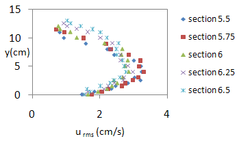Figure 8. Root mean square distribution of u'

Figure 9 shows that the region with the maximum values of turbulence intensity and maximum velocity gradient are coincident. In addition, the small aspect ratio (b/d) in table 1 does not affect the location of maximum velocity.

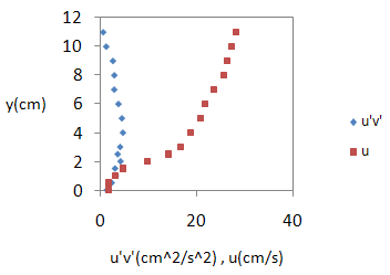Figure 9. Reynolds stress and velocity distributions

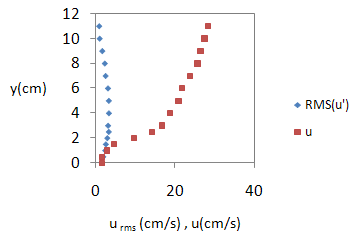Figure 10. Turbulence intensity and velocity distributions

4. Conclusions

The flow characteristics above submerged grass were studied under unfavorable pressure gradient. The flow velocity displays a clear inflection point due to vegetation. Such inflection point is not observed in gravel bed streams under unfavorable pressure gradient. The log law is valid above the vegetation cover in the inner layer and the defect velocity law fits reasonably well the outer layer data.The dimensionless pressure gradient parameter (β) follows Graf’s criterion (1998) for flow non-uniformity over the vegetated bed. The Reynolds stress and turbulence intensity distributions display a convex form which has been observed over gravel-bed streams.

Notation

u = Mean point velocity

u_* = Shear velocity

x = Longitudinal coordinate

y = Vertical coordinate

u_ave = Average velocity at a section

u_max = Maximum velocity

U_∞ = Surface water velocity

κ = von Karman constant

K_s = Roughness scale

C=constant of log law

δ = Boundary layer thickness

b/h = Aspect ratio

Fr = Froud number

δ_* = Displacement thickness of boundary layer

θ = Momentum thickness of boundary layer

β = Pressure gradient parameter

p = Pressure

τ = Shear stress

h = Water depth above the vegetation

τ_xy = Reynolds stress

u' = Turbulence intensity in the longitudinal direction

v' = Turbulence intensity in the vertical direction

ρ = density

u_rms = Root mean square of u'