Zahra Askari 1, Hossein Afzalimehr 2, Vijay P. Singh 3, Rohullah Fattahi 1
1Department of water engineering, Shahre-kord University, Shahre-kord, Iran
2Department of water engineering, Isfahan University of Technology, Isfahan, Iran
3Dept. of Biological and Agricultural Engineering and Zachry Department of Civil Engineering, Texas A&M University, USA
Correspondence to: Hossein Afzalimehr , Department of water engineering, Isfahan University of Technology, Isfahan, Iran.
| Email: |  |
Copyright © 2015 Scientific & Academic Publishing. All Rights Reserved.
Abstract
Velocity at the toe of structures, such as spillways, drops, and chutes, plays an important role in designing protective and control hydraulic structures. In this study, laboratory experiments were conducted to investigate velocity at an inclined surface with a height of 40 cm made up of galvanized steel in a flume 20 m long and 0.6 m wide. Using three different slopes, five different discharges and five kinds of roughness, 75 experiments were done. Comparison of measured and theoretical (measured by energy equation without considering losses) flow velocities showed that over the inclined bed, the correction coefficient of theoretical velocity for different Froude numbers varied from 0.87 to 0.88, reducing with roughness size. Roughness size, Froude number and the ratio of water head to the length of bed play a dominant role in the prediction of velocity.
Keywords:
Actual velocity, Theoretical velocity, Manning coefficient, Flow resistance
Cite this paper: Zahra Askari , Hossein Afzalimehr , Vijay P. Singh , Rohullah Fattahi , Prediction of Flow Velocity Near Inclined Surfaces with Varying Roughness, International Journal of Hydraulic Engineering, Vol. 4 No. 1, 2015, pp. 1-9. doi: 10.5923/j.ijhe.20150401.01.
1. Introduction
Flow in waterways with rough and inclined beds is complex because of the turmoil above and is often investigated through laboratory experiments. Flow resistance is among the important parameters in hydraulic calculations of flow in open channels. Velocity and shear stress are other characteristics of flow and their analysis is important in channels with rough beds. Due to the open flow surface, the pattern of secondary flows in open channels is different from that in closed channels. The secondary flows, including their shape and position, influence flow velocity, distribution of depth-averaged velocity, and shear stress. There is a relationship among the average velocity of flow, depth and slope of energy line, and the characteristics of waterways with constant bed. The relationship is often characterized by a resistance equation. There are different forms of this equations whose constants are determined for flows with constant bed.Flow resistance on rough and inclined beds has been a challenge in hydraulics. Resistance to flow in open channels is due to viscosity propulsion or pressure force created on wet surfaces. The various types of obstacles and roughness present on the bed and sides of rivers increase roughness in the flow path, cause loss of water energy, slows the flow, raises the river water surface, and generates flow in flat plains. Further, determination of flow resistance for calculating discharge, velocity, and sediment transport is essential. Calculation of water velocity near inclined surfaces, like the inclined spillways and drops, is needed to determine the hydraulic and geometric characteristics of downstream structures. Also, the coefficient of flow resistance is considered as a main factor in the simulation models of natural waterways. The coefficient is a function of velocity, depth, type of bed roughness, etc. Bradley and Paterka (1957) investigated the resistance on inclined surfaces and showed the relationship between the average velocity of flow and geometric, hydraulic and resistant parameters of waterways. Chezy (1775), Darcy-Weisbach (1875), and Manning (1890) are other frequently used relationships. The method of calculating coefficients reflecting the resistance derived from the roughness of flow profile is the most important issue in using these relationships; these coefficients are respectively recognized as the Chezy roughness coefficient (c), the Manning roughness coefficient (n), and thew Darcy-Weisbach coefficient and determining these coefficients has been a subject of considerable interest for hydraulic engineers. Based on statistical data related to the geometry and bed shape, Peterson (1969) and Bathurst (1987) conducted studies to obtain flow velocity and its relationship to flow resistance. To determine flow resistance regarding shear velocity and cross-sectional geometry, Keulegan (1938) investigated physical models. Some researchers considered methods to determine shear velocity and shear stress (Wolf, 1999; Kim et al., 2000; Thompson, 2003; Biron et al., 2004). Others theoretically investigated the development of bed shear velocity and shear stress based on specific assumptions on flow type (still/ turbulent, water depth), size of bed particles, flow distribution, and channel roughness (Kim et al. 2000). Shear velocity in flows with rough bed is usually determined by velocity profiles with overall depth, since there are ambiguities and complexities in the height of rough layer (Wilcock, 1996; Smart, 1999). The logarithmic profile method has been used in rivers with sandy bed to determine shear velocity (Nikora and Goring, 2000). Obtaining reliable information of velocity profile under certain circumstances, especially, in field is difficult. In this case, the shear velocity must be estimated from single point measurements. This method is commonly used in oceanographic studies. Kim et al. (2000) applied the method of Rowiski et al. (2005). The spectral method in a river estuary on the soft bed was also used and more studies were suggested with the use of the TKE method based on velocity measurements on two surfaces. Biron et al. (2004) conducted experimental studies on soft sands by using similar methods and they observed that the use of the logarithmic profile resulted in shear velocities that were considerably derived from other methods. Rowinski et al. (2005) compared these methods using flow experiments along with the beds reinforced with sand and found that the logarithmic profile method was not proper in these cases. They noted that due to irregularity in beds with coarse sand, using single point measurements to determine shear velocity was difficult. Thompson and Campbell (1979) conducted studies for determining the resistance in dam spillways. Smart and Jagy (1983) and Marcus et al. (1992) studied the relationship of flow resistance to discharge for rough beds. Einstein and Barbados (1952) studied the relationship between resistance and channel physics. Leopold et al. (1964) and Rose (1965) examined the resistance with speed in jumping pools. Lopez et al. (2007) examined the components of flow physical resistance in natural rivers to determine the flow resistance. Ganglie and Cutter (1877) developed a formula that the Chezy coefficient was a function of hydraulic radius, longitudinal slope, and wall roughness. Bazin (1897) proposed an equation to determine the Chezy coefficient depending on two parameters of roughness and hydraulic radius. Anderson and Straub (1960) conducted experiments in a flume with a length of 50 feet and a rough bed having particles with a thickness of 0.028 inches and presented an equation for determining the resistance coefficient. Bradley and Paterka (1957) presented a study, restricted to USBR, and showed a diagram as in figure 2 from which the ratio of the actual velocity to the theoretical velocity (the correction coefficient of velocity) can be estimated. According to these researchers, this diagram is a combination of experiments, measurements, and a limited amount of experimental data show the modeling in Shasta dam located to the north of California and Grand Cooley on Columbia River. Of course, this diagram has laboratory confirmation but it is more suitable for initial design; the theoretically used velocity is shown in figure 1.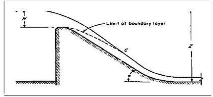 | Figure 1. Parameters provided in the velocity equation due to Bradley and Paterka (1957) |
These curves are applicable for steep slopes of H:V equaling 0.6 to 0.8. The curves of figure 2 show that the actual velocity of flow is closer to the theoretical velocity for increasing flow head. In other cases, when the height H (water head) and discharge are low, flow depth is low and due to friction, the resistance impact will be considerable. Usually, the flow is expected to change to a steady state before it falls with a great distance from spillway crest and this matter has been properly shown in the curves of figure 2.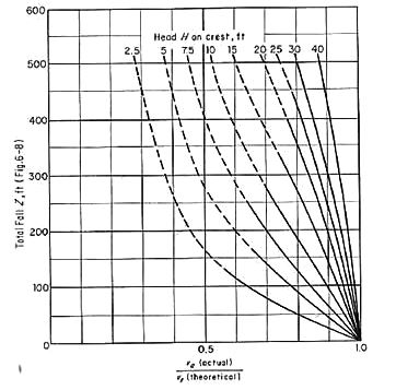 | Figure 2. Charts provided by Bradley and Paterka (1957) |
In this study, the velocity obtained by Pitot tube and the relationship presented by Bradley and Paterka (1957) has been respectively considered as actual and theoretical velocities; this relationship has been proposed as equation 1 and parameters have been introduced in figure 1. The relationship between the actual and theoretical velocities is presented as equation 2: 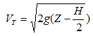 | (1) |
 | (2) |
where VR is the actual velocity measured by Pitot tube; VT is the theoretical velocity; and Cf is the correction coefficient. As is clear in Figure 2, the ratio of  against parameter Z and considering H (water head) on the spillway that Z is the difference of water height between upstream and downstream of the dam, is considered for determining the correction coefficient of velocity. In addition to the effect of these two parameters on the correction coefficient of velocity, other parameters, such as roughness, slope, and length of the inclined surface, Froude number, and the ratio of
  were studied and the impact of each one on this coefficient was examined. In open channel flows, the gravity force is a dominant force and Froude number (Fr) is the characteristic of open channel flow so Fr is one of the factors being studied. Resistance level or loss of energy depends on flow friction and the flow friction is dependent on surface roughness. Energy losses depend on the travel path of flow so the length of bed is a determinant on the inclined surface (L). In this study, our objective is to determine the correction coefficient of flow velocity by considering the effective parameters and the range of correction coefficient for different slopes and roughness and to propose the spectral relationships between parameters.
2. Methods
To achieve the objective of this study, experiments were done in a flume located in the hydraulic laboratory that has an inclined flume of a rectangular shape. The flume has a length of 20 m and a width and a height of 60 cm. The maximum discharge that can be pumped to this flume was obtained by a centrifugal pump that was 70 liters per second. To conduct the experiments, first an inclined surface made of galvanized plate with the ability to adjust slope was made and installed in the flume. For sealing the inclined surface and maintaining its stability against the pressure force of water, the glue proper and fixing screws were used. Studies were planned with three different slopes, five values of discharge, and five types of roughness. Thus, 75 experiments were done wherein five types of roughness were created by fastening the particles of wood and sand on the inclined surface consisting of flat surface, surface covered by chips of wood, and surfaces covered by three grades of 2 mm, 5.6 mm, and 6.3 mm. Also, three inclined surfaces with angles of 30, 45, and 60 degree were considered towards the horizon. Some images of implementing the inclined surfaces in the laboratory flume are shown in figures 4 and 5. To begin each experiment, the pump was turned on and besides adjusting the inlet discharge by volumetric counter, the velocity was measured by Pitot tube. According to flow depth, the velocity was measured at 1 to 12 points. Figure 3 shows the latitudinal profile of the actual velocity whose distribution is affected by the presence of secondary flows.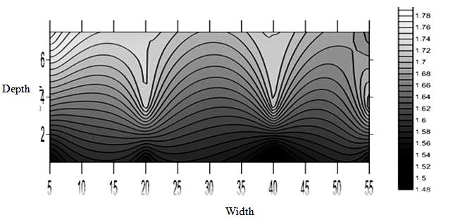 | Figure 3. Actual velocity profiles |
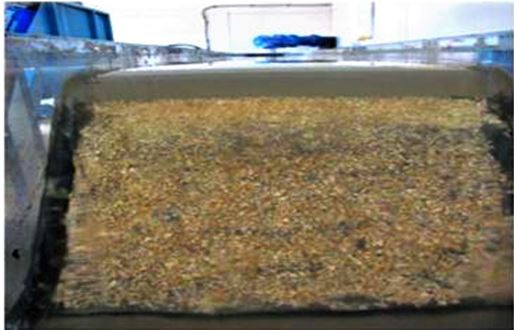 | Figure 4. Slope surface with wood excelsior |
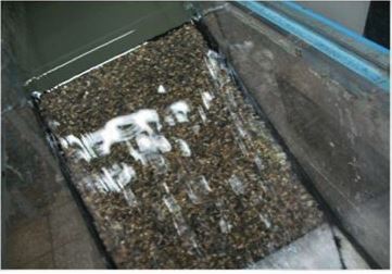 | Figure 5. Slope surface with sand of 5.6 mm |
In the experiments, the downstream valve was adjusted in a way that the water surface slope and the bottom of flume were exactly the same and this caused the steady flow to occur in the flume, so upstream and downstream conditions were controlled. Besides, the distance was considered as four times the width upstream and downstream to stabilize the upstream and downstream conditions. After calibrating the Pitot tube and applying the calibration coefficient, velocities were calculated as | (3) |
where k is the calibration coefficient, h is depth of the observed water, and g is the gravitational acceleration. The value of k was equivalent to 0.9 in this study.The roughness values from tables and using the following formula (Strickler) were obtained: | (4) |
where D50 is median particle size (mm), and n is the roughness coefficient.
3. Results and Discussion
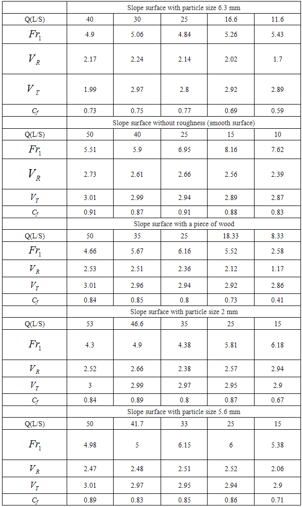
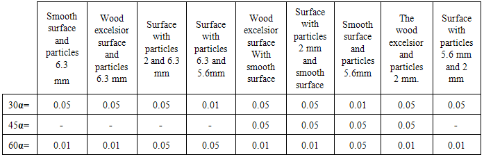
Flow velocity near the inclined surface was determined for two theoretical and actual states. The correction coefficient (Cf) was obtained by dividing the actual velocity by the theoretical velocity and the result is shown in Table 1. The SPSS software was used for data analysis and results showed that there was a significant relationship between Fr, n, and  parameters and the resistance coefficient, while there was no significant relationship between two other parameters, i.e., L and
  and the correction coefficient for velocity.
Table 1. Velocity measured for slope of 30° and 5 different types of roughness
 |
| |
|
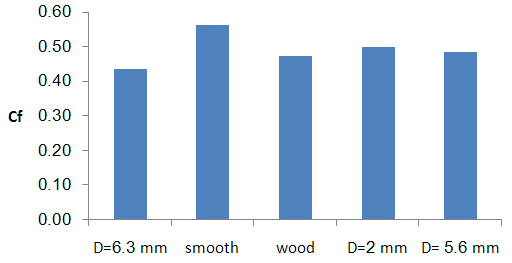
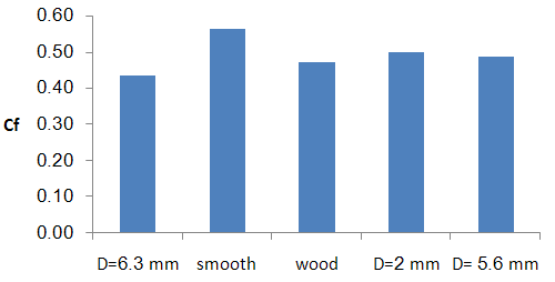
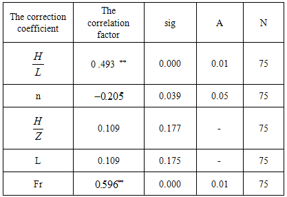
The roughness influenced somewhat the correction coefficient of velocity. As expected, results showed less the roughness, more the correction coefficient and vice versa. The least amount of resistance was observed on the inclined surface with roughness of 6.3 mm. Regarding the Pearson test (this correlation coefficient was adjusted based on the covariance of two variables and their deviations), if both variables are in relative and interval scale, the Pearson correlation coefficient was used. The significance test of the correlation coefficient was used to assess the confidence level of this correlation. It was investigated whether the relationship between two variables was random and they were independent of each other. Also, statistics (sig) or P-Value related to the observed correlation must be smaller than error. Between the Cf and  parameters, the null hypothesis was rejected, because the value of the test statistics was less than alpha (H0 means lack of relationship between the parameters) so there was correlation and the Pearson correlation coefficient was equal to 0.493; according to this test, the correlation coefficient was about -0.205 for n and Cf. The correlation coefficient with the Froude number was 0.596. In Figs. 6 and 7, it is clear that the angle or (L) has no effect on the coefficient (Cf). Regarding the effect of two parameters, i.e.,
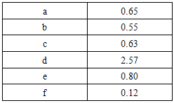
  and roughness (n), on the coefficient (Cf) with equation 6, the above two coefficients were obtained to determine this coefficient (Cf). The coefficients of this equation in the range of experimental conditions used in this study are presented in Table 3. Also, eq. 5 that is a nonlinear relationship with 6.47% error was obtained by using the solver in Excel; the coefficients of this relationship are presented in Table 2.
 | (5) |
 | Figure 6. Effect of roughness on the correction coefficient at an angle of 30 degree |
 | Figure 7. Effect of roughness on the correction coefficient at an angle of 45 degree |
Table 2. Coefficient of equation 5
 |
| |
|
Table 3. Table of statistics information
 |
| |
|
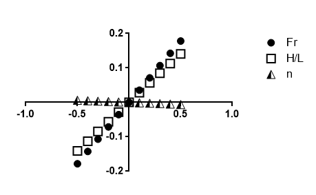 | Figure 8. Sensitivity analysis |
Table 3 shows the effective parameters on the correction coefficient of velocity and the significance level.Equation 6 is the relationship of the correction coefficient of velocity with effective parameters derived from linear regression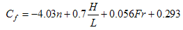 | (6) |
Fr is the Froude number.  is the ratio of water head to the overall height. Sensitivity analysis, based on equation 6, showed that the value of this coefficient showed the least sensitivity to parameter n and the most sensitivity to the Fr parameter. The above material is obtained from the relationship and its coefficients are deduced. Figs. 9 and 10 are graphed to investigate the correction coefficient of velocity and parameters without
  and Fr.
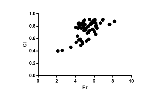 | Figure 9. Scatter plot of velocity correction coefficient and Fr |
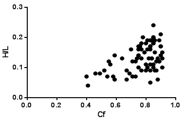 | Figure 10. Scatter plot of velocity correction coefficient and  |
These figures show that the correction coefficient of velocity increases with increasing Froude number and the ratio of  . In other words, the difference between theoretical and actual velocities reduces. Table 3 shows that the correlation is significant at the 1% significance level between these two parameters and the correction coefficient of velocity near the inclined surface. The type of roughness, the Froude number, and the ratio of
  have a significant impact on the correction coefficient; these parameters were not considered by Bradley and Paterka (1957). The reason for different values of this coefficient in different slopes is that if the angle of the inclined surface is 45 degree, the development of the boundary layer in the downstream path of spillway will increase and when the whole profile is not filled by the boundary layer, the turbulent flow is not fully developed (Henderson, 1966). In a mutual comparison of roughness, this characteristic of the inclined surface with a 45-degree slope and the developing boundary layer led to different results compared to 30 -and 60-degree slopes. The influence of the Froude number in the case of different roughness values on the correction coefficient was studied and results showed that on flat inclined surfaces and with the Froude number greater than 5, the correction coefficient changed between 0.83 to 0.91; on the inclined surface with wood chips, the Froude number was close to 1 and the range of correction coefficient changed between 0.4 to 0.85 (figure 10).
4. Conclusions
Results of this study show that the velocity near inclined surfaces is not independent of the characteristics of the inclined surface and hydraulic conditions of flow. Comparison of measured and calculated velocities for surfaces with different roughness values shows that there is an opposite relationship between the absolute roughness and the correction coefficient of velocity; also the difference between theoretical and measured values of velocity shows that  has a significant impact on the flow resistance but the slope of the inclined surface does not have any effect on the correction coefficient. Due to the complete development of boundary layer, the mutually significant relationship between different roughness values with a 45- degree angle was less than that with 30 and 60- degree angles. Also, the nonlinear relationship of parameters that influence the correction coefficient of velocity with a high correlation coefficient (0.9) is justified to predict the actual velocity. Statistical results of the SPSS software reveal that relationship between the parameters of relative roughness,
  , and the Froude number with the correction coefficient of velocity show that these parameters are among the dominant and controlling parameters to predict the theoretical velocity. Using the results of this study, it is possible to design downstream structures like still basin with a higher safety factor and a better approximation of velocity.
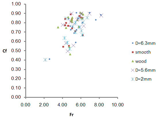 | Figure 10. Effect of correction factor on the Froude number |
Table 3. Surface roughness of between2 to 2different angles
 |
| |
|
Notation
Fr Froude number (-)n Manning roughness coefficient (-)Cf Velocity coefficient (-)H/L Ratio of water head to slope surface lengthZ Total water head between upstream and downstream (m)H/Z Ratio water head to total head (-)LSlope surface length (m) Theoretical velocity (m/s)
 Real velocity (m/s)g Gravity acceleration
  k Calibration coefficient (-)
 Median grain size of bed (m)
References
| [1] | Bradley. J. N Paterka, A.J.1957. The hydraulic design of stilling basins. Proc. Am. Soc. Civil. Engrs, Vol.83 pp.1401-6. |
| [2] | Bathurst, J. C. (1987). Theoretical aspects of flow resistance in gravel-bed Rivers, edited by R. D. Hey, J. C. Bathurst, and C. R. Thorne. 83-105, John Wiley. |
| [3] | Keulegan GH (1938)." Laws of turbulent flows in open channels", J. Res. Nat. Bureau of Standards, Vol.21, No.6, 707-741. |
| [4] | Wolf, J. (1999). The estimation of shear stresses from near-bed turbulent velocities for combined wave-current flows.” Coastal Engineering, 37, 529–543. |
| [5] | Thompson, C. E. L., Amos, C. L., Jones, T. E. R., and Chaplin, J. 2003. The manifestation of fluid-transmitted bed shear stress in a smooth annular flume; A comparison of methods. J. Coastal Res., 19(4), pp.1094-1103. |
| [6] | Biron, P. M., Robson, C., Lapointe, M. F., and Guskin, S. J. 2004. Comparing different methods of bed shear Stress estimates in simple and complex flow fields. Earth Surface Processes and Landforms, 29, pp. 1403-141. |
| [7] | Kim, S-C, Friedrichs, C.T., Maa, JP-Y, Wright, L.D. 2000. Estimating bottom stress in tidal boundary layer from Acoustic Doppler velocimeter data. J. Hydr Engrg, ASCE, 126(6), pp.399-406. |
| [8] | Wilcock PR. 1996. Estimating local bed shear stress from velocity observation. Water Resource Research 32: 3361- 3366. |
| [9] | Rowinski PM, 2005. Shear velocity estimation in hydraulic research. Acta Geophysica 53:567-583. |
| [10] | Smart, G.M. 1999. Turbulent velocity profile and boundary shear stress in gravel bed rivers. J. Hydrraul. En.106, pp 106-115. |
| [11] | Nikora, V. I., D. Goring. 2000. Flow Turbulence over fixed and weakly mobile gravel beds. J Hydraul. Eng. 126(9): 679-690. |
| [12] | Einstein, H. A. (1942). “Formulas for the transportation of bed-load.”Trans. Am Soc. Civ. Eng., 107, 561–597. |
| [13] | Leopold, L.B., M.G. Wolman, and J.P. Miller. 1964. Fluvial Processes in Geomorphology. W. H. Freeman and Co. San Francisco. |
| [14] | Rose. H Reid.L.1935.Model Research on spillway crest, civil engineering vol.5 chaps 14. |
| [15] | Henderson. F.M. 1966. Channel controls. (Open channel flow). pp 181-189. |
| [16] | López F. and García M. H. 2001, Mean flow and turbulence structure of open channel flow through non-emergent vegetation. Journal of Hydraulic Engineering, Vol. 127, No. 5, pp. 392–402. |
| [17] | Strub. G Anderson.A.G.1960. Experiments on self-aerated flow in open channels. 456 p. |
| [18] | Comiti F. Mao L. Wilcox A. Whol E.E. Lenzi M. 2007. Field-derived relationships for flow velocity and resistance in high-gradient streams. |
| [19] | Barani, G. 1996. Hydraulic of open channels (1st edition). ShahidBahonar University of publication. |
| [20] | Birami, M. 2009. Structures of transferring water (8th edition). Isfahan University of publication. Isfahan, Publishing center; No. 35. Department of Engineering; 23. |
| [21] | Shafaei Bajestan, M and Bahrami Yarahmadi, 2013. M. Experimental study of roughness coefficient of Manning in open channels with coarse bed. Journal of Research of the Ministry of Agriculture, Vol. 25, No. 2: 91. |
 Abstract
 Reference
 Full-Text PDF
 Full-text HTML