Siake A.1, Koueni-Toko C.2, Djeumako B.1, Tcheukam-Toko D.3, Soh-Fotsing B.4, Kuitche A.5
1Department of Mechanical Engineering, ENSAI, University of NGaoundéré, P N’Déré, Cameroon
2Department of Renewable Energy, ISS, University of Maroua, Maroua, Cameroon (CMR)
3Department of Energy Engineering, IUT, University of NGaoundéré, NGaoundéré, Cameroon
4Department of Mechanical Engineering, IUT- FV, University of Dschang, Bandjoun, Cameroon
5Department of Electrical, Energy and Automatism control Engineering, ENSAI, N’Déré, CMR
Correspondence to: Tcheukam-Toko D., Department of Energy Engineering, IUT, University of NGaoundéré, NGaoundéré, Cameroon.
| Email: |  |
Copyright © 2014 Scientific & Academic Publishing. All Rights Reserved.
Abstract
Numerical analysis was performed for a draft tube flow of a hydraulic turbine. Special attention has been paid for the friction effect through the flow inside the complex geometry of the draft tube, and for the interaction between the vortex structures and the draft tube volute. A draft tube affected could have a large significance on the performance prediction of hydraulic turbines, even on the efficiency of a hydroelectric center. The turbulent model has been applied a standard κ-ε two equations model and the two-dimensional Reynolds Averaged Navier–Stokes (RANS) equations, are discredited with the second order upwind scheme. The SIMPLE algorithm, which is developed using control volumes, is adopted as the numerical procedure. Calculations were performed for a wide variation of runner velocities. The results reveal that with increasing of the runner velocity, the velocity decreases and the static pressure increases, justifying the total recuperation of kinetic energy at the draft tube outlet. Comparison of numerical results with the experimental data available in the literature is satisfactory.
Keywords:
Hydraulic turbine, Draft tube, Hydrodynamic, Velocity field, Pressure field, Hydroelectricity, CFD
Cite this paper: Siake A., Koueni-Toko C., Djeumako B., Tcheukam-Toko D., Soh-Fotsing B., Kuitche A., Hydrodynamic Characterization of Draft Tube Flow of a Hydraulic Turbine, International Journal of Hydraulic Engineering, Vol. 3 No. 4, 2014, pp. 103-110. doi: 10.5923/j.ijhe.20140304.01.
1. Introduction
The utilization of the hydraulic force in the domain of the electricity production has long been majority; it has started in antiquity with mills of water. The techniques permitting the exploitation of hydroelectric resources have beneficed important progress during the XX century, in the scope of projects construction of the hydroelectric center of great speed. Through their size, their precision and their efficiency, the equipments of these hydroelectric center and especially hydraulics turbines arrived in first plan of realization. The hydraulic turbine is a mechanic dispositive which is used to transform potential energy and the kinetic energy of water, in mechanic energy. This will then be transformed into electric energy by an alternator. There exist two categories of hydraulics turbine. The turbine of action, which do not constitute a draft tube and function with the kinetic energy of water, and the turbine of reaction, which function with the pressure difference and the energy pressure. With the increasing coast of energy and the high demand of green energy, hydraulic turbine of thin height of falls such as Francis and Kaplan turbines, are those targeted as being economically profitable. They are constituted of distributor, of volute, of runner and draft tube. The draft tube permits the recuperation of excess water kinetic energy coming from the runner and converts it into energy of static pressure.Many studies on the draft tube flow have been done. Marjavaara [1], carried out a numerical study to show that the draft tube have an important rule on the global efficiency of a hydraulic turbine. According to Cervantes et al. [2], draft tubes are of great interest for turbines of thin height of fall like Kaplan turbines, since the draft tube efficiency increases with the decreasing of the height of fall. Andersson [3], had done an experimental study in the draft tube cone. He demonstrates that for small height of fall and high output, loses in draft tube are considerably high and can go up to 50%. Labrecque [4], did a study on the conception of the axial turbine. He demonstrated that the augmentation of the performance of hydraulic turbine pass by a good knowledge of the flow in the turbine. Gubin [5], carried out an experimental study on the flow in the draft tube of a hydraulic turbine. He shows that the efficiency of the turbine of reaction can be significantly affected by the performance of its draft tube. Ciocan et al. [6], effectuated a study on the flow at the entrance of draft tube by the LVD and PIV methods. They noticed that this flow at the entrance is characterized by eddies, wakes and the non uniformity. Mauri [7], effectuated a numerical study in addition to experimental study, to demonstrate that oscillatory flow in draft tube evolves in a progressive manner up to end. Susan-Resiga et al. [8], showed that oscillatory flow at the runner outlet of a hydraulic turbine influences the flow in the draft tube.This confirms the complexity of the flow in a draft tube of a hydraulic turbine. The knowing of the evolution of hydrodynamic parameters of the flow such as the velocity and pressure in the draft tube, can contribute to the amelioration of its efficiency and by then, the performance of the hydroelectric center. According to Čarija et al. [9], a numerical study of the flow with the method RANS, and using the model of turbulence k-ε, permits to well predict the flow in a draft tube. According to Duprat [10], the great gradient pressure coupled to the form of the draft tube, created unfavorable conditions on the stability of the flow which generate then the detachment of boundary layer. This present work consists in doing a numerical study of the dynamic field in a draft tube of a hydraulic turbine. It will help to well understand the influence of hydrodynamic parameters on the efficiency of the draft tube.To lead well this study, we are going to present the mathematical formulation and the computation procedure employed. These methods have permitted to calculate, the velocity and pressure fields in the draft tube, and the velocity profiles at five sections, by using a model of bi-dimensional turbulence, isotropic and stationary.
2. Mathematical Formulation and Computation Procedure
2.1. Assumption of Calculation Domain
Our work of simulation is done through a draft tube of hydraulic turbine placed inside a hydroelectric dam. The geometry and the dimensions of draft tube have been chosen in conformity with the experimental works of Anderson [3], represented by the figure 1 bellow, showing the different measurements points. These works have been done for a functioning mode of 60% of total load, which means the mode near the best possible efficiency. The table 1 bellow represents the functioning parameters of hydraulic turbine according to the experimental works of Anderson [3], that we used for this present numerical work.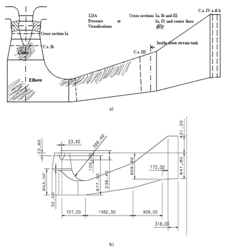 | Figure 1. Geometry and dimensions of draft tube (Anderson [3]); a): front view; b): dimensions |
Table 1. Functioning parameters proposed by Anderson [3]
 |
| |
|
2.2. Governing Equations
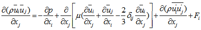
The monophasic turbulent flow in the draft tube is described by a set of non-linear partial differential equations expressing the physical laws of conservation between the velocity and pressure at each point of the flow: the Navier-Stokes equations. To these equations, we add the equation of turbulent kinetic energy and that of its dissipation rate like proposed by Launder and Spalding [11]. Solving these equations will reveal features such as pressure and dynamic fields, and axial and tangential velocity profiles. | (1) |
 | (2) |
The relation (1) is a continuity equation, and (2) is the equation of the quantity of movement conservation in which:l the left term represents the convective transport;,l the first term on the right represents the forces due to the pressure;l the second term on the right represents the forces of viscosities;l the two last terms on the right represents the forces generated by the turbulence.The means equations lead to the appearance of the double correlation terms of the velocities fluctuations. They come from the non-linearity of conservation equations. These terms are called Reynolds stress , and translate the effect of turbulence on the evolution of the means movement, giving the equations systems open by introducing supplementary unknowns terms. The closure problem is resolved through the hypothesis of Boussinesq:
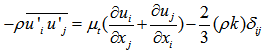 | (3) |
We are going to use for our resolution, the model of turbulence k-ε standard proposed by Fluent [12], which is a model enough used: | (4) |
To determine  , we have to calculate the two variables k and ε. The equations of kinetic energy turbulent and its dissipation rate give us the following relations bellow:For the kinetic energy turbulent
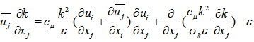 | (5) |
lthe term at the left represent the variation of the kinetic energy turbulent;lthe first term at the right represents the production of kinetic energy turbulent;l the second term at the right represents the diffusion;l the last term at the right represents the dissipation.The dissipation energy equation is given by the following relation: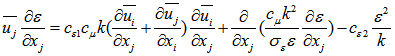 | (6) |
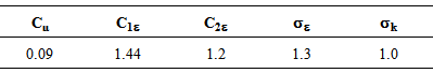
Where, Cµ, Cε1 and Cε2 are empirical constants; σε and σk are respectively the turbulent Prandtl numbers relative to k and ε. The values of these constants proposed by Jones and Launder [13], are represented on table 2 bellow. Table 2. Empirical constants proposed by Jones and Launder [13]
 |
| |
|
2.3. Computation Procedure
The transition from physical domain to the numerical domain begins with the generating mesh geometry by a preprocessor. Then import this into a computational code for the iterative solution of equations to determine the values of variables on each node of the mesh. The segregated solution method was chosen for the resolution of turbulence model and governing equations. Governing equations were discredited with the control volume technique. For the convective and the diffusive terms, a second order upwind method was used while the SIMPLE (Semi Implicit Method for Pressure Linked Equations) procedure was introduced for the velocity-pressure (Patankar, [14]). The convergence of the numerical calculation is checked by examining the evolution of relative residuals in each governing equation for a convergence criterion of 0.001%. The stability of the iterative process was carried out by relaxation coefficients associated with the velocity, pressure, κ, ε and μt. The Standard Wall-Functions were used to take into account the effects of friction near the wall. Three mesh distributions have been tested to ensure that the calculated results are grid independent. The similar method was already used by Tcheukam-Toko et al. [15].
3. Results and Discussion
3.1. Generating Mesh Geometry
The figure 2 below represents the computational domain meshed with the code GAMBIT. The grid distribution is a set of quadrilateral cells (uniformly structured mesh). The calculations will use the software Fluent [12]. The mesh is very uniformly fine near the wall and around the runner outlet, where the velocity gradient is large. The grid distribution impacts the computation time and the number of iterations required for the solution converge. The choice of the mesh size of 90,000 cells is a good compromise and the results that will be presented later are those of this mesh size. The no-dimension variables are: | (7) |
 | (8) |
The no-dimension runner velocity and rate of flow are respectively N+ = 140 and Q+ varying from 0.984 to 0.996.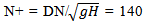 | (9) |
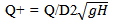 | (10) |
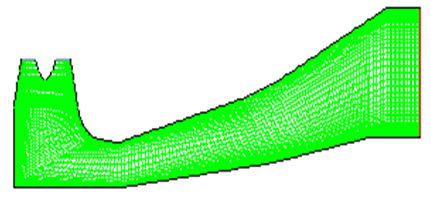 | Figure 2. Grid configuration |
3.2. Pressure field
The figure 3 below represents the dynamic pressure field in the draft tube. We observe a maximal dynamic pressure at the entrance of draft tube cone, generated by the oscillatory flow outing from the runner. At the draft tube cone outlet, we observe an important loss of dynamic pressure which evolves up to the downstream from the draft tube elbow. This loss of pressure is generated by the draft tube geometry. The pressure decreases along the draft tube diffuser and become very low at the discharge port of draft tube. 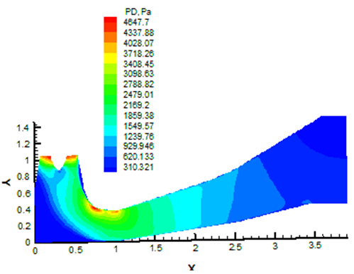 | Figure 3. Dynamic pressure field |
The figure 4 bellow represents the static pressure field in the draft tube. We observe the low static pressure at the entrance of draft tube cone generated by the runner velocity. This loss of static pressure allows a good flow dynamic inside the elbow. At the inferior region of elbow, the static pressure is increasing while it is decreasing at the superior region. At the downstream from the elbow, the static pressure increases slowly to the maximum value up to end.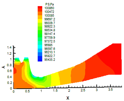 | Figure 4. Static pressure field |
3.3. Velocity Field
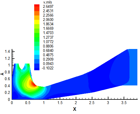
The figure 5 below represents the axial velocity field in the draft tube. We observe that the axial velocity is maxima inside the draft tube cone. We observe also a strong velocity gradient inside the cone, generated by the draft tube elbow (90°), and the oscillatory flow. Many separated flow regions and flow recirculation zones, appear inside the draft tube. The axial velocity flow is decreasing along the draft tube diffuser in progressive manner up to end, justifying the total recuperation of kinetic energy before the discharge port of draft tube. The figure 6 below represents the tangential velocity field in the draft tube. We observe that the tangential velocity is low at the entrance of draft tube cone. A recirculation zone appears near the draft tube cone outlet. This velocity increases in the superior region because of elbow geometry. The tangential velocity starts to decrease from the entrance of draft tube diffuser up to end.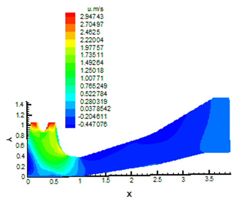 | Figure 5. Axial velocity field |
 | Figure 6. Tangential velocity field |
3.4. Velocity Profiles
The runner velocity generates the centrifugal forces which could affect many hydrodynamics parameters allowing the performance degradation of the hydraulic turbine. To well understand this phenomenon, we are going to describe the runner velocity influence on the axial and tangential velocities profiles at five sections (Ia, Ib, II, III, IV), of draft tube named as follow: Ia: Draft tube cone inletIb: Draft tube cone outletII: Draft tube elbowIII: Draft tube diffuserIV: Draft tube outlet
3.4.1. Axial Velocity Profiles
The figures 7a, 7b, 7c, 7d, and 7e below represent the axial velocity profiles respectively at the sections Ia, Ib, II, III, IV of the draft tube, for different runner velocities. The figures 7a & 7b show that the axial velocity amplitude increases with the velocity runner and remains positives in the draft tube cone. These results are in concordance with the experiments results of Ciocan et al. [6].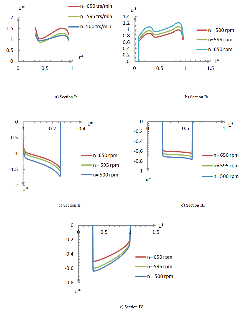 | Figure 7. Axial velocity profiles for different runner velocities at the sections Ia, Ib, II, III, & IV |
The amplitude axial velocity is varying with the draft tube radius. This variation is generating by the vortexes structures outing from the runner. The figures 7c, 7d & 7e show the negatives values of velocity which become lower in progressive meaner up to end. The total kinetic energy is recuperated in the draft tube despite the increasing of runner velocity. This is generated by the increasing section of draft tube diffuser. The influence of runner rotation on the axial velocity affects the losses pressure and the recuperation coefficient. This result is the same obtained by Ruchi et al., [16].
3.4.2. Tangential Velocity Profiles
The figures 8a, 8b, 8c, 8d, and 8e below represent the tangential velocity profiles respectively at the sections Ia, Ib, II, III & IV of the draft tube, for different runner velocities. The figures 8a and 8b show an increasing of the tangential velocity amplitude with the increasing of the runner velocity, but it remains periodic. This velocity is positive with the high amplitude values, generated by the runner rotation which created some vortexes structures in the draft tube cone. These results are in concordance with the results of Ciocan et al. [6]. The figure 8c shows a linear variation of the tangential velocity, with a positive and a negative zone traducing the fluid recirculation. The figures 8d & 8e show the negatives values of velocities traducing the total dispersion of vortexes at the draft tube outlet.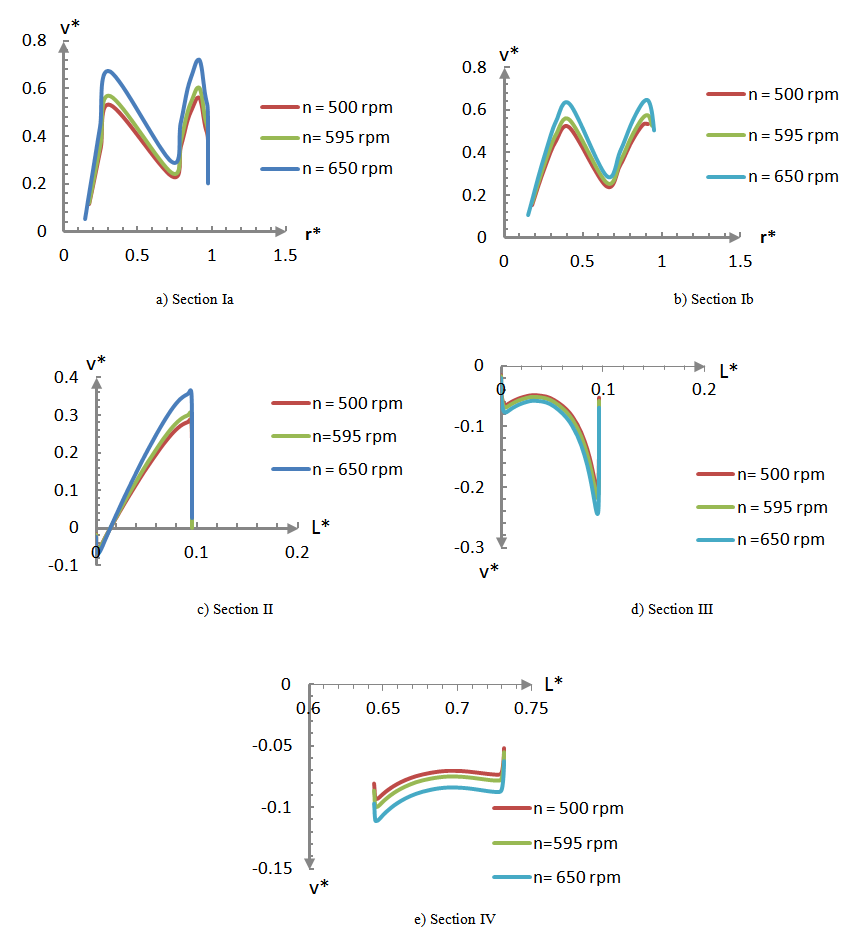 | Figure 8. Tangential velocity profiles for different runner velocities at the sections Ia, Ib, II, III, & IV |
4. Comparison of Results
Anderson [3], had carried out the experiments data for one runner velocity (595 rpm), at the sections Ia and Ib of the draft tube cone. The figures 9a & 9b bellow represent the axial velocity profiles respectively at the sections Ia and Ib. 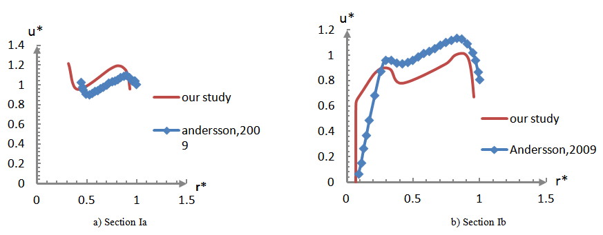 | Figure 9. Axial velocity profiles for 595rpm; a): section Ia; b): section Ib |
We observe that our numerical results and the experiments data are in good concordance. We observe also a recirculation zone at the center of draft tube cone. The increasing of axial velocity with the radius is linear and periodic with two maxima and minima. Its decreases at the region near the wall. The figures 10a & 10b bellow represent the tangential velocity profiles respectively at the sections Ia and Ib. We observe that our numerical results have a low difference with the experiments data. This difference is generated by the wall effects inside the draft tube that the simulation 2D does not take in account. The tangential velocity increases at the entrance of draft tube cone (section Ia), showing a wake zone at the draft tube cone outlet (section Ib).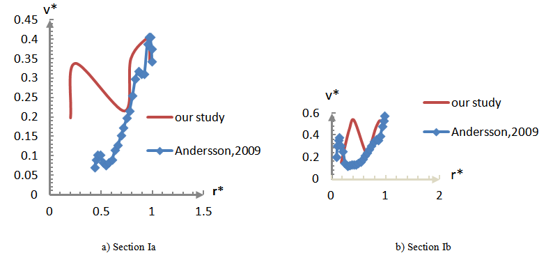 | Figure 10. Tangential velocity profiles for 595 rpm; a): section Ia; b): section Ib |
5. Conclusions
We have presented the pressure and velocity fields showing the separate zones and the zones of recirculation which influence the flow in the draft tube of a hydraulic turbine. We have also presented the velocity profiles on different sections of the draft tube. The comparison of our results with the experimental results of Anderson [3], show a good agreement of the axial velocities. But, the tangential velocity profiles show a difference which could be explained by the wall effects, that our simulation code 2D do not take in account. The velocity profiles that we have obtained on three other sections II, III, IV of the draft tube (i. e. zones difficult to get access in experimental), are likely. The dynamic pressure is too small at the discharge port of draft tube. These qualitative considerations illustrated that the draft tube has an important rule on the hydraulic turbine performance.
Nomenclature
D: tube diameter (m)x: axial coordinate (m)y: vertical coordinate (m)L: draft tube length (m)v: vertical velocity (m/s)u: longitudinal velocity (m/s) : mean of longitudinal velocity (m/s)
 : longitudinal velocity fluctuation (m/s)g: gravitational acceleration (m. s-2)p: pressure (N/m2)
Greek symbols
ν: kinematic viscosity (m. Kg-1. s-1)ρ: density (kg. m-3)μ: dynamic viscosity (m. Kg-1. s-1)κ: turbulent kinetic energy (m3. s-2)ε: Dissipation rate (m3. s-3) : Krönecker symbol
 : Turbulent viscosity (m2/s)
 : Shear stress
References
| [1] | Marjavaara B. D., (2006). CFD driven optimization of hydraulic turbine draft tubes using surrogate models, Doctoral Thesis, Lulea University of Technology ISSN: 1402-1544, Sweden. |
| [2] | Cervantes M., Andersson U., and Löfgren H. (2010), turbine-99 unsteady simulations-validation, 25th IAHR Symposium on Hydraulic Machinery and Systems, Timisoara Romania. |
| [3] | Anderson U., (2009). Experimental study of sharp-heel Kaplan draft tube, Doctoral Thesis, Lulea University of Technology, ISBN: 978-91-86233-68-6, Sweden. |
| [4] | Labrecque Y., (1993). Conception de turbines axiales, Projet de fin d'Etudes, Université de Laval, France. |
| [5] | Gubin M. F., (1973). Draft tubes of hydro-electric stations, Amerind Publishing Co, New Delhi; India. |
| [6] | Gouin P., Deschenes C., Iliescu M., Ciocan G., (2009). Experimental investigation of draft tube flow of an axial turbine by LDV. 3rd IAHR International Meeting of the Workgroup on Cavitations and Dynamic Problems in Hydraulic Machinery and Systems, Bern, Czech Republic. |
| [7] | Mauri S., (2002). Numerical simulation and flow analysis of an elbow diffuser, PhD. Thesis, École Polytechnique Fédérale de Lausanne, Communauté Helvétique. |
| [8] | Susan-Resiga R. F., Ciocan G., Anton I. and Avellan F., (2006). Analysis of the swirling flow downstream a Francis turbine runner, Journal of Fluids Engineering, 128, pp. 177–189. |
| [9] | Čarija Z., Mrša Z. and Dragović L. (2006), turbulent flow simulation in Kaplan draft tube, 5th International Congress of Croatian Society of Mechanics; Zagreb, Croatia. |
| [10] | Duprat C., (2010). Simulation numérique instationnaire des écoulements turbulents dans les diffuseurs des turbines hydrauliques en vue de l’amélioration des performances. Thèse de Doctorat, Université de Grenoble, France. |
| [11] | Launder B. E. and Spalding, D., (1974). The numerical computation of turbulent flow computational methods, Applied. Mechanical Engineering, Vol. 3, pp. 269-289. |
| [12] | Fluent (2006). User manual 6.3.26. |
| [13] | Jones J. and Lauder B. E., (1961). A Single Formula for the Law of the Wall, Journal of Applied Mechanics, Vol. 28, No. 3: 444-458. |
| [14] | Patankar S.V., (1980). Numerical heat transfer and fluid flow, McGraw Hill, New-York. |
| [15] | Tcheukam-Toko, Mokem-Chetchueng M., Mouangué R., Beda T., Murzyn F., (2013). Characterization of Hydraulic Jump over an Obstacle in Open-channel Flow. International Journal of Hydraulic Engineering (IJHE), 2(5), 2013, 71-84. |
| [16] | Ruchi K., Vishnu P., and Mitrasen V., (2012). Design optimization of conical draft tube of hydraulic turbine, International Journal of Advances in Engineering, Science and Technology ISSN: 2249-913x vol. 2 no. 1. |
 Abstract
 Reference
 Full-Text PDF
 Full-text HTML