1. Introduction

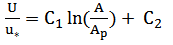
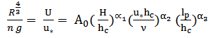
Ecological and aesthetic values have become an integral part of modern river management, and therein natural riverbank and floodplain vegetation plays major role. In recent years, river restoration has become an accepted practice in many countries [1]. In this regard, softer alternatives to earlier engineering solutions, such as bioengineering, are being increasingly preferred. Of fundamental importance in river restoration is the assessment of flow resistance caused by vegetation [2].

Vegetation, in general, is a controlling factor in the interaction of flow, erosion and geomorphology in rivers and may cause difficulties in hydraulic design. Vegetation along rivers and in floodplains consumes a great amount of energy and momentum from the flow, and is often found to be in the region with most roughness [3]. The transfer of momentum causing shear stress on channel walls influences the main channel flow and floodplains as well as erosion and the stability of banks [4]. Masterman and Thorne (1992) pointed out that bank vegetation is a key factor in reducing flow velocity [5].

Interactions between flow and vegetation are complex and depend on environmental factors and plant characteristics, such as mean flow velocity, turbulence, channel morphology, water temperature, plant morphology, age and size, and the spatial distribution of plant patches [6].

Many investigations have already been undertaken to describe the relationship between flow resistances, Manning’s n, or drag coefficient (C_d), with the type and spatial distribution of vegetation. Analytical and experimental studies of vegetation-related resistance to flow depend on relative submergence [7]. Also, plant characteristics, such as leafs and bending, may have an important influence on the flow resistance ([2], [8]).

The chart below shows that flow resistance depends on many factors.

The definitive quantitative relation between flow resistance and controlling parameters (predictor parameters) is a long-standing problem in hydraulics and remains unclear as yet [9]. A rigorous approach for deriving hydraulic resistance relationships is based on the integration of the double-averaged (in time and space) Navier–Stokes equations [10]. However, it is not an easy task to quantify the contribution of all predictor parameters in the flow resistance equation by Navier–Stokes equations.

Among simplified approaches which are currently applied, two methods are promising. The first method was suggested by Kouwen et al. as follows:

(1)

Where

Cross sectional mean velocity = U

Shear velocity = u_*

Figure 1. Chart showing parameters affecting flow resistance estimation

Total cross sectional area of the flow = A

Part of the total cross sectional area occupied by vegetation = A_p

Coefficients depending on vegetation properties = C₁ and C₂

Equation (1) was originally derived using the logarithmic formula of velocity distribution above vegetation canopy uniformly covering the bed. Subsequent tests, showed that for a range of hydraulic conditions, this equation approximates experimental data reasonably well [11].

In this relationship, the ratio of A / A_p is considered for a straight section with a bed uniformly covered by vegetation, whereas this relation can be changed for the channels which are not fully covered by vegetation as follows:

(2)

In which

Mean flow width = W

Mean flow depth = H

Mean width of vegetation = W_c

Mean averaged height of the vegetation canopy = h_c

The second method was suggested by Carllow (2005) [12]

(3)

Where

Hydraulic radius = R

Manning coefficient = n

Gravity acceleration = g

Plant shoot length = l_p

A coefficient depending on vegetation density = A₀

Empirical exponents = α₁, α₂ and α₃

Parameters of the resistance coefficient can be computed using the following relations:

(4a)

(4b)

(4c)

Where n is the Manning coefficient, S is the water slope, U is cross sectional average flow velocity, C_d is drag coefficient, C'_d is a bulk drag coefficient, which is a lumped parameter based on the total frontal area of vegetation in channel reach, i.e., projected plant area per unit volume ([13], [14]).

The objective of this study is to investigate the relationship between flow resistance and vegetation parameters in a gravel-bed river with vegetated banks, and find an empirical relation. Also, using the collected data in this study, the application of the log law and the equation (3) are investigated.

2. Experimental Setup

A reach of Babolroud River was selected for field experiments. The river is located near the city of Babol in north of Iran, near the Caspian Sea. The reach was 250 m long with 13 measured cross sections where 11 cross sections of which are with vegetation on banks and 2 cross sections of which are with bare banks. Figure 2 presents a plan of selected reach.

Figure 2. Plan of the selected reach

The median grain size of bed material was determined by the Wolman method (1954) equal to D₅₀ = 30.58 mm with a standard deviation of 1.6. The standard deviation shows that the bed material are uniform because the uniformity coefficient (D₆₀/D₁₀₎ was 2.05. Figure 3 presents the grain size distribution for Babolroud River [15].

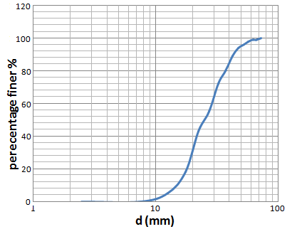Figure 3. Grain size distribution of bed material

The vegetation covers along the banks of the selected reach is similar to rice, 24-54 cm high, showing considerable flexibility. As shown in Figure 4, the vegetation cover for the most part was under water surface, showing a plant inclination factor between 1.5-3.

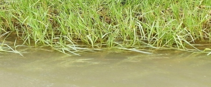Figure 4. Image of vegetation along river banks

At each cross section, five velocity profiles were measured; one velocity profile at the central part of the reach, two velocity profiles along each river bank, and two velocity profiles between the central axis of the reach and river banks. Sixty five velocity profiles were measured for 13 cross sections and for each profile 10-15 point velocity values were measured. A butterfly current meter (Figure 5) was used to measure the point velocity in the vertical direction from the bed to the water surface. Each point velocity measurement was taken during for 50 seconds with three repetitions to get an accurate average.

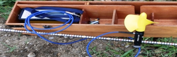Figure 5. Current-meter used in this study

The friction slope was calculated using the Saint Venant equation as follows:

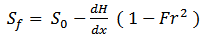(5)

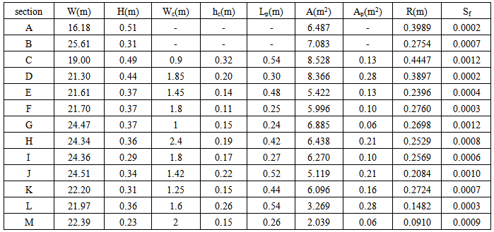
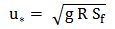
Where S₀ is the bed slope, is the flow depth variation and Fr is the average of Froude number at each cross section. The range of width and depth of the reach is from 17.5 to 25.6 meters and 0.14 to 0.65 m, respectively.

Discharge was calculated by using the continuity equation Q = A × V, where A is the cross section area, and V is the weighted velocity in each section.

Table 1 presents a summary of experimental and calculated data for 13cross-sections along the selected reach, where W_c and h_c present the weighted values.

No vegetation cover was observed at the sections of A and B, that is why no value was reported for W_c, h_c, L_p and A_p at these sections.

Table 1. Summary of measured and calculated data

The Reynolds number (Re) and Froude number (Fr) were computed and their values showed that the flow was turbulent and subcritical. Shear velocity was calculated by using the Saint Venant equation (5) as follows:

(6)

The range of flow discharge (Q) was from 1 m³/s to 10 m³/s during the fieldwork along the selected reach (table 2). The values of τ in table 2 presents the bed shear stress.

Table 2. Summary of hydraulic parameters

3. Results

3.1. Velocity Distribution

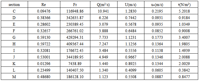
Considering the range of river width in table 1, the aspect ratio (W_c / h_c) changes with an interval of 26-100 with an average of 80. Figure 6 shows measured dimensionless velocity profiles in which the maximum flow velocity occurs at the water surface for the bare banks sections, however, near the vegetated banks the dip phenomenon is observed in which the maximum flow velocity is below the water surface. Also, the application of the log law is presented for each velocity profile in Figure 6.

Figure 6. Velocity distribution and log law application for bare banks and vegetated banks sections

Nezu (1985) concluded that the maximum velocity occurred at the water surface for the aspect ratio larger than 5 which is consistent for the bare bank sections. However, for vegetated bank sections, even if W_c/h_c> 5, the maximum flow velocity occurs under the water surface. The reason for such behavior is the interaction of vegetation with secondary currents which causes the vertical as well as lateral components of velocity to be activated. This causes lateral velocity to move from the water surface towards the central axis and the vertical component of velocity forces the velocity to move toward the bed leading the maximum velocity to occur under the water surface. In addition, the velocity distribution near the vegetated bank (Figure.6) reveals that a small aspect ratio is not the main cause for occurrence of the maximum velocity below the water surface, but vegetated shear layers produced such a pattern. The presence of vegetation on the river banks changes flow structure. Afzalimehr and Dey (2009) found that vegetation cover changes uniform flow to non-uniform flow, showing a nonlinear distribution of Reynolds stress [16]. In other words, it is excepted that Reynolds stress distribution display a linear distribution for uniform flow, however, vegetation forces a nonlinear distribution.

In open channel flow, velocity profile can be presented on the basis of the universal log law:

(7)

Where, u = mean point velocity, u_* = shear velocity, y = distance from the bed, ҡ = the Von Karman constant, which is taken 0.4, k_s = roughness scale, which is considered equivalent of D₅₀ and C₃ = a constant. Figure.6 shows that the log law does not apply over the whole flow depth from the bed to the water surface, however, depending the location of velocity across the river, it applies for the near bed data with different commencement levels. Considering Figure.6, it is found that the thickness of the log law zone for the bare bank profiles are larger than vegetated banks. This can be explained by generation of turbulence by vegetation, forcing a reduction in thickness of log law. In either 2D or 3D flows, as pointed out by Afzalimehr and Dey (2009), the presence of secondary currents (the dip phenomenon) does not influence the log-law validity in gravel-bed channels. A deviation of the velocity profile from the log-law in the outer layer (far from where y/h>0.2) is considered to flow over gravel bed with or without vegetated banks. The reasons for velocity profile deviation from the log law line are the near bed acceleration resulting from flow contraction over the leading edge of gravel particles and invalidity of mixing length over the whole flow depth of river. Figure 6 shows that vegetation on river banks does influence the thickness of log law zone where the log-law is applicable, however, the log law can be applied in different distances from vegetated banks in gravel-bed rivers.

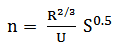
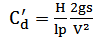
3.2. Flow Resistance Estimation

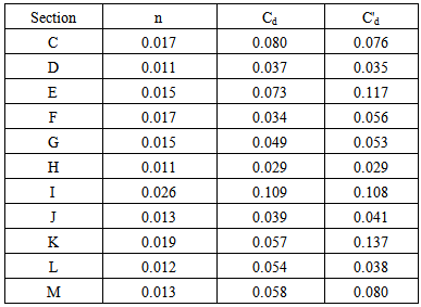
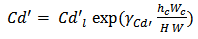
The flow resistance was determined using equations (4). Results of the weighted values of the Manning coefficient (n), drag coefficient (C_d) and bulk drag coefficient are presented in table 3.

Table 3. Calculated values of Manning coefficient, drag coefficient and bulk drag coefficient

Considering the existing literature on the flow resistance, the influential vegetation parameters to flow resistance can be presented as relative roughness , plant inclination factor , and areal vegetation cover [17].

In the studies of Kouwen (1969), Watson (1987), Barky et al. (1992), Champion and Tanner (2000) and Green (2005a), the site average relative roughness was adequate to predict the flow resistance. Therefore, it was selected for this study ([9], [11], [18], [19]).

Using a statistical analysis of resistance coefficients and , it was found that the best correlation with a range of R² 0.733 revealed an exponential function.

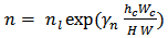(8a)

(8b)

The relationships n = f (hcWc /HW), can be best approximated by exponential functions n=nl exp (nhcWc /HW), where subscript ‘l’ indicates limits of the resistance factors when (hcWc /HW) → 0, and γ_n, is a coefficient.

The results of Green (2005) and Nikora et al. (2008) showed a relation between Manning’s n and Ap / A with R² = 0.744 and R²= 0.82, respectively, but our data showedR² = 0.733 for n, and R² = 0.517for drag coefficient (Figure 7) [20, 21].

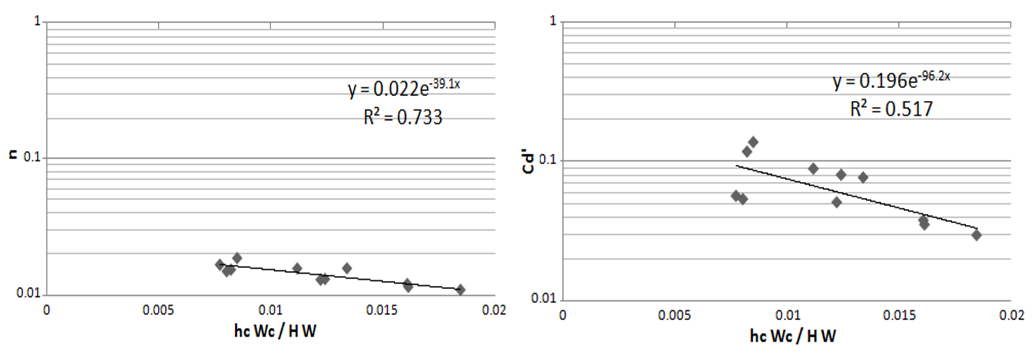Figure 7. Exponential relations of flow resistance

Using the software of SPSS and equation 3, a nonlinear regression was used to compute unknown coefficients α₁, α₂ and α₃ (equation 6). The quantity of A₀ was assumed 1 since it had not been measured before.

(9)

For grass-type vegetation with low stem density, Carllow (2005) found that α₁ = 1.168, α₂ = 0 and α₃ = -0.861 [11].

When this quantities were replaced for α₁, α₂ and α₃ the quantity of and were achieved as A₀ that drawing the plot for cross sections was in the form of linear sub contrariety with R² = 0.943 (figure 8).

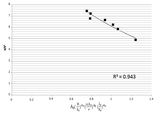Figure 8. Flow resistance presentation

As table 3 indicates the calculated Manning coefficient (n) varies from 0.011 to 0.026 in this study. On the other hand, Afzalimehr et al., (2010) found a range of 0.043 to 0.056 to flow in natural channels with vegetated bed [7]. However, using vegetation cover over the bed, they found a range of 0.023 to 0.029 for (n). The reason for small values of n in this study is the large aspect ratio, showing the larger aspect ratio, the smaller is Manning coefficient. In addition, the interactions of relative roughness, Reynolds number and plant inclination factor play important impacts on flow resistance estimation in vegetated banks rivers.

4. Conclusions

The following conclusions are drawn from this filed study:

1. The aspect ratio varies from 26 to 100 with an average of 80 showing the larger aspect ratio, the smaller is Manning coefficient.

2. The maximum flow velocity occurs at the water surface for the bare banks sections, but near the vegetated banks the dip phenomenon is observed and the maximum flow velocity occurs below the water surface.

3. Vegetation on river banks affects the thickness of log law zone where the log-law is applicable, showing this law can be applied at various distances from vegetated banks in gravel-bed rivers with different commencement levels.

4. The relation between the Manning roughness coefficient (n) and average relative roughness was found to be exponential, with the coefficient of determination of 0.733.

5. For grass with low stem density, the relation between relative velocity and characteristic parameters of relative roughness, Reynolds number and plant inclination factor was significant with the coefficient of determination of 0.943. More data are required to calibrate and validate the findings of this research.

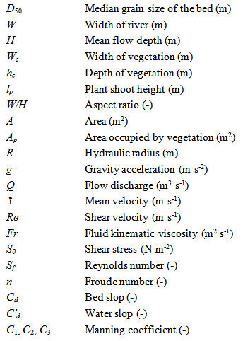
Notation