Carl Y. H. Jiang
Faculty of Science, Engineering and Built Environment, Deakin University, Victoria, 3216, Australia
Correspondence to: Carl Y. H. Jiang , Faculty of Science, Engineering and Built Environment, Deakin University, Victoria, 3216, Australia.
| Email: |  |
Copyright © 2014 Scientific & Academic Publishing. All Rights Reserved.
Abstract
The research provides a novel approach in modelling flood by means of effectively integrating remote sensing imagery with the corresponding digital elevation model. The seamless correlation between remote sensing imagery and digital elevation model produces a very powerful advantage in application of hydraulic engineering. In this research, based on such correlation, the large scale flood area can be easily discovered according to the elevation of water surface in local lake. The spatial and geometric data and information of lake which are obtained by combining individual advantage of remote sensing imagery and digital elevation model provide not only a proof to explore flood channel but also data to model arbitrarily selected flood channel. In the further modelling, the values of hydraulic parameters can be easily gained without any local measurements. In the process of calculation, the equation of calculating longitudinal velocity at an arbitrary cross section is based on the equation used to calculate the superelevation of channel. The equation is modified by introducing new concept parameter and easily to apply. The values for the required parameters such as superelevation and curvature radius are easily gained, calculated and treated as natural characteristic parameters for any shape cross section to calculate the longitudinal velocity which is termed as the critical overflow velocity. The hydraulic properties at each cross section are calculated by using this mean longitudinal velocity. In the final approach, the distribution of the longitudinal velocity at an arbitrary cross section was also explored by means of the feature of continuity of flow. Due to a conversion coefficient being introduced, the transversal distribution of longitudinal velocity is easily discovered and displayed. Several ignored hidden factors are uncovered and the error can be compensated for by using the conversion coefficient. The result is consistent with the real cases.
Keywords:
Flood modelling, Floodplain, Open channel, Hydraulics, Remote sensing imagery, Digital elevation model, Digital image processing
Cite this paper: Carl Y. H. Jiang , Model and Forecast Flood by Integrating Remote Sensing Imagery with Digital Elevation Model: A New Approach for Flood Modeling, International Journal of Hydraulic Engineering, Vol. 3 No. 2, 2014, pp. 35-60. doi: 10.5923/j.ijhe.20140302.01.
1. Introduction
Flood is one kind of natural disaster. It belongs to the domain of open channel research. Because flood happens every year in the world, consequently people have been investigating it for over thousand years to control and protect it. However, in modern hydraulic engineering, hydraulic engineers are still using some empirical equations to design hydraulic project. Because empirical equations relies on many experiments in order to obtain effective and accurate coefficients to meet local topographical features. That results in massive cost in experiments and time. Accordingly, it is necessary to explore a novel manner to reduce the cost, improve the accurateness and effectiveness of project. In this research, author proposes a new manner to model flood and forecast it utilizing a landscape remote sensing imagery and the corresponding digital elevation model (DEM). Advantages of Combining Two Different Data ResorcesRecently, although many researchers [1-10] have already paid their attentions to using data gained by modern technology such as remote sensing imagery, digital elevation model (DEM) and Lidar, in practice these valuable data have not been fully used. Hence, those valuable data were separately used into individual research fields. Superficially, different data generated by different modern technologies have individual feature and advantage. They look correlation for the same investigated object on the Earth, but such correlation is remained at superficial level. Actually, mathematically speaking, there are hidden correlations amongst those data. They are built on the same mathematical platform – matrix. The functionality of matrix acts as a bridge to link and integrate multidiscipline. On the other hand, individual data can be further developed and utilized combining them with individual knowledge in different research field. The combined features and functionalities from different data sources become very powerful and flexible in discovering many unknown facts. This approach can be applied into the wide range application including hydraulic engineering. In hydraulic engineering, the advantage of such approach can be not only shown in individual development but also further extended to integrating pre-treated data with the functionalities of other package such as HEC-RAS, which is a package especially used in modelling open channel. In the case of modelling floodplain, if the inserted data is well pre-processed, it could be more accurate and effective for its post-process [11]. The advantage of new approach is briefly introduced above. Because there is a big different approach in applying the existing data into different research field, the detailed application in modelling flood is to be introduced and discussed in a series of subsections so as to fully understand the advantage of this new approach.
1.1. Features and Tasks of Research
The new approach has the following unique features in modelling flood. 1. Find local water level by means of discovering the elevation of the existing lake. The geographical location of lake was already captured by landscape satellite and stored into remote sensing image. The maximum depth of lake and the elevation of free surface in lake are obtained by means of remote sensing imagery and DEM using linear indexing technique.2. Because the local elevation of water is discovered, its value is treated as a threshold to seek for the area to be inundated when storm happens.3. Discovered area can be further used to model flood by increasing its elevation in this area.4. Extract partial channel as an investigated object to model flood.5. The partial flood channel is divided by several cross sections6. Each cross section is then used to study hydraulic properties when fluid (water) flows through each of them.7. Because this is new approach, some existing equations have to rebuild on the basis of approved theories of fluid. Several coefficients are to be introduced.8. The transversal distribution of longitudinal velocity is to be investigated. Meanwhile, in order to clearly demonstrate how the values of some common parameters are achieved using new approach, the basic concepts used in hydraulic engineering are to be briefly reviewed. Furthermore, some most important concepts of new approach, thus the technique of integrating remote sensing imagery and digital model (DEM) are briefly introduced as well, and one more example in detecting river in remote sensing imagery is supplied to demonstrate.
1.2. Select Geographic Location
The selected geographical location for modelling flood is (-36°70'10" S, 146°44'30" E; -36°83'60" S, 146°71'00" E) where natural disasters such as bushfire and flood often happened in Victoria, Australia (see Figure 1). Figure 1 is a satellite imagery captured by LANDSAT (supplied by NASA). The lake and natural channel is easily distinguished from it. 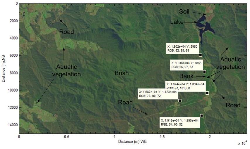 | Figure 1. Selected geographic location in remote sensing imagery (472×933) for modeling flood |
The flood was usually caused by large storm. In terms of distribution of aquatic vegetation, the inundated area is obviously discovered. The flood impacted the existing roads in this area. On the other hand, it is also found that the terrain in this area is complicated.
2. Basic Concepts in Studying Open Channel
Investigating flood belongs to the domain of open-channel. There are several parameters used to discribe variation of the channel and the quantity change of flow in it. The standandard definations of them are already termed in some text books and hand books [12-16].In order to esily and clearly illustrate applications and developments in this field. Some relevent hydraulic concepts and definations are reviewed as follows. 1. Flow area (A): the flow area is the cross-sectional area of the flow taken normal to the direction of flow.2. Top width (T): the top width of a channel is the width of the channel section at the water surface.3. Wetted perimeter (Pw): the wetted perimeter is the length of the line that is the interface between the fluid and the channel boundary perimeter.4. Hydraulic radius (Rh): the hydraulic radius is the ratio of the flow area (A) to the wetted perimeter (Pw), which is termed as  | (1) |
5. Hydraulic depth (Dh): the hydraulic depth is the ratio of the flow area (A) to the top width (T) ), which is termed as | (2) |
6. Superelevation (Δe): the rise in the elevation of the water surface at the outer channel boundary above the mean depth of flow in an equivalent straight channel, because of centrifugal force in a curved channel (see Figure 2). 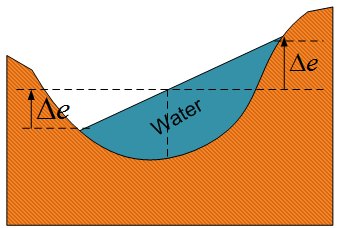 | Figure 2. The schematic of super-elevation |
The superelevation can be assessed by the following equation [17].  | (3) |
Where r is curvature radius, ε is a correction factor to calculate the total rise in water surface due to superelevation and standing waves under different conditions of flow, cross section and curve type. It can be selected by either 0.5 or 1.0. For the tranquil flow, ε=0.5. Equation (3) can be derived by the momentum equation in the transversal direction [14]. This concept is very important in this research, which is to be discussed more in the subsections. Modelling flood is based on this concept.7. Specific energy (E): if the datum is selected at the bottom of channel, the sum of Z+P/ρ is constant and equal to the depth of flow, the specific energy of an open-channel flow is defined as follows. | (4) |
Where d is the depth of flow, V is mean velocity of flow, g is gravitational acceleration (9.80 m/s2 in Victoria), ζ is the kinetic energy correction coefficient respectively in the context. ζ ranges 1.0 to 2.0 [13] to correct the one-dimensional kinetic energy unevenly distributes across the cross section. In the case of flood, ζ can be up to 2.0 or more.If the mean velocity V is defined as | (5) |
Where, Q is flow rate, and then equation (4) can be written as | (6) |
8. Critical depth (dc): assume that flow is uniform and the shape of channel is rectangular, then ζ=1, ∂A/∂d=T. Due to continuity, the velocity V and the flow rate q per unit width can be defined as follows respectively,  | (7) |
Then equation (4) is rewritten as  | (8) |
The depth of flow d in equation (8) as a function of E is plotted and shown in Figure 3. It can be discovered that when d⟶∞, E→ line d=E, and d→0, E→∞. The asymptote moves to the left or right side as the flow rate Q decreases or increases respectively. Therefore, two limbs of asymptotes are formed meanwhile and distinguished by the critical point A, thus the limb AB (subcritical flow) and AC (supercritical flow) are formed by accompanying with distinguished Froude number (Fr). 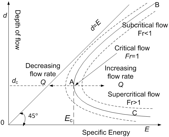 | Figure 3. Relationship between subcritical flow, critical flow, supercritical flow and specific energy and depth of flow |
The minimum depth of flow for a specified flow rate Q is then obtained by 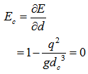 | (9) |
Accordingly, the critical depth (dc) is expressed as  | (10) |
9. Froude number (Fr): the Froude number is the dimensionless ratio of the inertial and gravitational forces, thus  | (11) |
As indicated in Figure 3, when the flow is at critical point A, Fr =1as V=√gDh.If the slope and the kinetic energy correction coefficient ζ are considered, equation(11) is usually rewritten as | (12) |
Where, θ is the slope angle of bed.Froude number (Fr) is one important parameter to discribe how the inertial and gravitational force act on the motion of fluid. When Fr<1, thus √gDH>V, the gravitational force plays a dominant role in the motion of fluid. Oppositely, when Fr>1, the inertial force is dominant. When Fr = 1, it represents a critical point to determine which force is in dominant state when extra conditions such as variation of flow rate Q exert upon the process of conversion (see Figure 3). Furthermore, when Fr=1 appears, the corresponding critical depth (dc) and the minimum specific energy (thus Ec) to pass the flow rate Q can be found.10. Total energy (H): the total energy is composed of three terms, which can be expressed by Bernoulli equation as follows | (13) |
WhereZ is the elevation of the point above a reference plane.P is the pressure at the chosen point, thus over an arbitrary datum at a vertical plain. ρ is the density of fluidIn this case, the term P/ρ is pressure head, the term V2/2g is velocity head.ζ is kinetic energy correction factor. For uniform flow, ζ=1.0. Equation (13) is also expressed as the following equation to describe the velocity varying across the section (see Figure 4). | (14) |
Whered is the depth of flow.Z0 is bed elevation based on a given datum. However, in this research, it can be directly replaced by the corresponding elevation of DEM.Analogous to a form of energy per unit mass, d cosθ is the pressure head, Z0 is the potential head and V2/2g is the kinetic energy head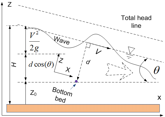 | Figure 4. The schematic of illustrating relationship total head line with other parameters in open channel |
11. Celerity (C): the celetity characterizes the propagation of wave relative to the fluid motion. It can be discribed by the following equation if the slope angle θ and kinetic energy correction factor ζ are taken into account. | (15) |
It is caused by gravitational force; therefore celerity is velocity of gravity wave.Under supercritical flow conditions (see Figure 3) thus d<dc or Fr>1, a wave cannot move upstream as the velocity of flow (V) exceeds the wave celerity (C), thus V>C. However, When d>dc, Fr<1 or V<C, the flow is in subcritical state, the wave can propagate upstream against the flow, and upstream areas are in hydraulic communication with the downstream areas [12].12. Empirical equations applied in open channelTraditional investigating flood is based on empirical equations (such as Chezy’s, Manning’s, and Darcy’s). The frequently used equation is Manning’s equation, for uniform flow rate Q, which can be shown as the following form (SI units) [13]. | (16) |
Where n is Manning’s resistance coefficient and S is channel longitudinal slope. In 1889, Robert Manning, a professor at the Royal College of Dublin established this equation, which was developed from the equation initially created by Antoine Chezy during in the period 1768–1775 [13]. However, most difficult to use Manning equation is to find reliable n. Although many handbooks [12-15] and textbooks provide a lot of empirical equations to estimate n such as  | (17) |
With conditions: ,Obviously, its application must rely on a lot of indirect experiments to confirm various parameters. That certainly causes errors. Therefore, a new approach of integrating remote sensing imagery and DEM is proposed by author and introduced in the following sections.
3. Methodology
In the following subsections, some vital concepts and prameters used in modelling flood are to be introduced in terms of the physical and hydraulic characters of flow and the feature of terrain.
3.1. Defining Some Parameters Used in Modelling Flood
Feature of Natural ChannelFor most natural channels, the main feature of them is not straight and has many irregular shapes of cross sections, thus gradually and spatially varied channel (GSVC), in other words, mathmatically speaking the natural channels are consisted of a series of continous curves with different curvetures and curveture radius at any arbitary cross-sectional sections. The floodplain usually starts to overflow from the existing natural channel because it is the lowest level of storing water at local place when storm is encountered. Analysis of Force Balance Water overflow in channel is directly caused by unbalanced sum of forces, therefore analysing force balance is quite necessary and important. In classical physics, although there are several forces such as gravitational force (F1), drag force or boundary shear force(F2) and force related to momentum of flow or inertial force (F3) exerting on elementary volume of fluid when fluid passes a certain curved channel section with a mean velocity (V) and curvature radius (r) (see Figure 5), whether the fluid overflows the bank relies on the balance of two coupled horizontal forces: centripetal force (F5) and centrifugal force (F6) are achieved. The balance of F5 and F6 is maintained by another reaction force (F4) from one side wall of channel while surging force against it. Once such a balance of sum forces is broken, water overflows bank. 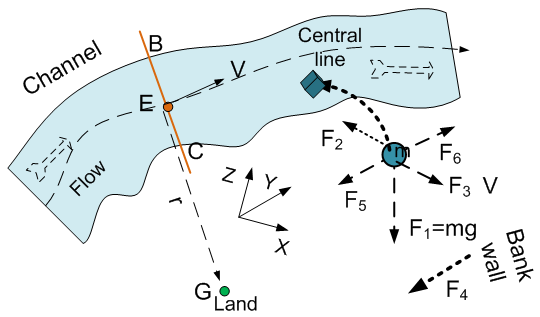 | Figure 5. Sketch of water flow at curved channel |
According to to Newtonian second law, the centripetal force F acting on the object having mass m, tangtal velocity V at curvature radius r can be expressed by the following relation: | (18) |
The balance of sum forces exerting on one volume element of fluid have direct relation with the magnitude of velocity V, curvature radius r and the density of fluid ρ.Process of Forming Overflow In flooding, due to an amount of upstream water flowing into areas downstream, thus large Q (inlet flow rate or discharge rate) under an extreme weather such a storm, the balance between upstream flow rate and the flow rate of discharge downstream determines how fast the level of water rises in channel. Figure 6 illustrates this process. In Figure 6, the point E is defined as centre point of width T of top water surface. The subscript n indicates the variation of parameters with respect to time like time series. At initial stage, water flows in flood channel at very low level (e.g. the point J), which is impossible to cause flood rapidly. With increasing upstream flow rate Q, the magnitude of parameters (V, A and T) become larger and larger. Finally the highest level of flow reaches up to the maximum height point of one side bank such as point B in Figure 6. Then, overflow from both side banks occurs. The difference between maximum heights at both side banks can be described by the superelevation (∆e) (see Figure 2). In other words, there is a critical velocity for each section of curved channel.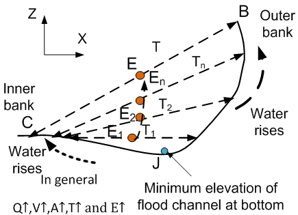 | Figure 6. Schematically illustrates water rises in open channel |
Mathematically speaking, such a critical velocity of overflow for most natural channels could permanently exist because there is a difference of elevation between both side banks for any arbitrary section. Critical Curvature Radius of OverflowIn terms of equation (3) and (18), to find critical velocity of overflow, a vital parameter: the curvature radius (r) must be confirmed firstly. The curvature radius r can be obtained by the following approach. a) Assume the point B and C is the point of maximum height at both side ranks in one arbitrary cross section respectively (see Figure 7). 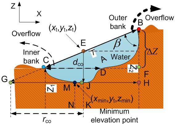 | Figure 7. Water overflows out of both side banks |
b) Extend line BC infinitely, usually a point G can be found in a remote place unless the point B and C is located at the same level (elevation).c) There must be an angle: β between the line BC (thus top water surface T) and the vertical line BH which must be perpendicular to the horizontal line CF being drawn from the point C. If the point B and C are located at the same level, then β=90° and the distance of the point G approaches to infinite. d) Another interested vertical line is EJ, which must be parallel to the vertical line BH as well as perpendicular to the horizontal line CF and GH. The point E is that which locates at the centre of T. In result, the difference of the height between point B and point C can be easily gained by the following relation: | (19) |
Where, Z1 and Z2 represent the elevation of DEM at the point C and B respectively. The depth of water dco, when water rises to the critical state to overflows from both side banks (see Figure 7), is then expressed as follows. | (20) |
Where Zt is the elevation of the mean point located in the centre of top water (T), which is to be discussed in the following subsection. Zmin is the minimum elevation indicated by the point M at the bottom of flood channel in any arbitrary cross section. In this approach, the elevation of the point J corresponding to the point E is replaced by the elevation Zmin at the point M so as to find the curvature radius(r). Such a treatment does not cause too much error because the line JK is parallel to the line MN.Consequently, the critical overflow curvature radius rco (the subscript co denotes critical overflow in the context) is obtained by the following correlated equations.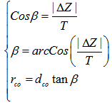 | (21) |
Obviously, the maximum or minimum height Z at both side banks, hence, elevations of two side banks varies along longitudinal channel, but it does not affect calculation of angle β because the absolute sign∥ is applied into elevation difference. Because ∆Z for any cross section is a natural feature, the rco approaches to it too.Critical Velocity of OverflowIn above section, the critical curveture radius of overflow rco is already confirmed. The critical velocity of overflow in this research can be intepreted as that the extreme speed of flow before fluid exceeds the minimum height of channel bank. In terms of illustration of Figure 6, Figure 7 and equation (3), it is easy to find the potential correlation.Water overflows from both side banks (see Figure 7). That means that the elevation of water in the flood channel to be increased is at least as two times height as ∆e (or ∆Z). This target is achieved by increasing flow rate. According to the principle of original derivation (see Figure 2), the kinetic energy correction coefficient ζ should be included because the mean velocity is tangtal speed. That leads to | (22) |
Although two parameters ε and ζ were already introduced by different researchers to investigate the behaviour of flow, it is difficult to determine their values in practice. In order to simplify the case, only one parameter ω is introduced into and termed as a flow rising parameter, which is a time-varied dimensionless variable. And then equation (22) is rewritten as the following form. | (23) |
And assume ω = 1 as an extreme value to describe the case that overflow happens at both side banks at any cross sections. Parameters for Transversal Distribution of Longitudinal Velocity in Flood ChannelThe critical overflow velocity Vco supplied by equation (23) is treated as a mean longitudinal velocity at any cross sections, however, which does not tell how the real longitudinal velocity distributes in the transversal direction and how fast it varies in vertical direction. This topic should be considered further.Physically speaking, the velocity V at any spatial point can be resolved into three components (Vx, Vy and Vz) (see the velocity V at the point D in Figure 8). The velocity Vx can be ignored because it is towards both side banks, however, which is one of factors causing uneven distribution of longitudinal velocity in transversal direction at one cross section.In order to know how the real longitudinal velocity (Vco,y ) distributes in the transversal direction (x), the subscript y denotes the critical overflow velocity in longitudinal (y) direction, the equation (23) is required to reassess. As discovered from it, the surface width (T) is a main parameter in achieving this target. Once its distribution is known, the transversal distribution of Vco,y is then confirmed. To know it, the point has to start from the bottom of flood channel, thus the wetted perimeter (Pw). At the nth section, its length Ln between two sections: Bn-1 and Bn (see Figure 8) is known based on the knowledge of DEM. Its slope angle αn is easily calculated by means of the geometric features of DEM. The nth surface width Tn can be obtained by the following correlation. | (24) |
Where, angle β is already gained by equation (21).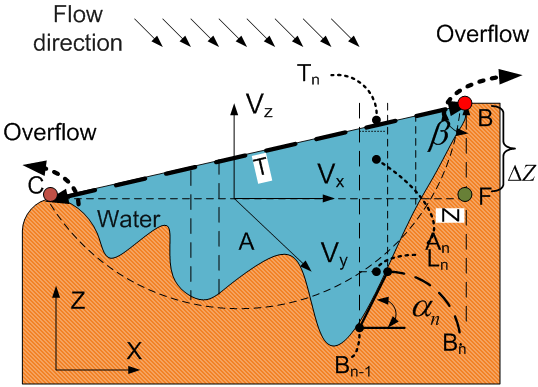 | Figure 8. Schematically illustrate velocity components distribute across flood channel section |
More about Flow Rising ParameterIn fact, it is difficult to assess how the longitudinal velocity varies as assessing how fast the water rises from the bottom of flood channel. However, according to equation (21), the parameters ∆Z, T and rco can be accurately confirmed or assessed by using the data supplied by combining remote sensing imagery with DEM. Therefore ω becomes an adjustable variable based on the calculated value of critical velocity of overflow Vco, which is obtained when ω is set as one at the first trial at any cross sections. Then, it can be used to estimate the variation of velocity of flow in flood channel as the magnitude of flow rate Q is increased by adjusting the range of ω. Hence, the task of describing the complicated process of flood rising in the flood channel (see Figure 6) could be replaced by setting up the range of ω, which is to be described as follows. It is assumed that the longitudinal velocity Vy(t) in flood channel with respect to time( t) at one arbitrary section can be expressed as follows. | (25) |
Where, the variable t is time, the subscript y denotes longitudinal direction. ω (t) may be thought as a time series or a specified function of time. There are two simple cases to be considered about flow rising parameter ω(t), which happens at any shape cross section in flood channel. 1) If flood is gradually and spatially varied flow (GVSF), the flow rising parameter ω(t) may be written as a linear function and increased with one constant ratio. However, its range should be larger than zero and less than one. The interval is decided by how fast the flow rate (Q) grows up at one selected cross section. Its expression is like equation (25).2) If flood is a quickly and spatially varied flow (QVSF), the flow rising parameter ω(t) may be written as a logarithmic form and increased with respect to time. Equation (25) is then modified as  | (26) |
With  ,
,  Determine Transversal Distribution of Longitudinal Velocity in Flood Channel using DEM Although the magnitude of velocity variable Vy (t) which varies in the longitudinal direction(y) is described by using ω(t) in equation(25) and (26), it is still difficultly applied into practice. However, in terms of the continuity of fluid, at one specified time (t) such as at the time of critical overflow and the total cross sectional flow area (A) consisting of n subsections is assumed, the flow rate (Q) in the following equation (27) and (28) can set up their correlation.
 | (27) |
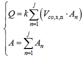 | (28) |
Where, k is a dimensionless conversion coefficient between equation (27) and (28).In the DEM based practice, the approach could be simpler. The mean longitudinal velocity can be calculated by using equation (23) if the elevations of both side banks and the value of ω(t) are specified. Then the value of k is obtained by assessing whether the product of the averaged sum of longitudinal velocity distributing in the transversal direction and the assigned value of k is close to the mean longitudinal velocity or not. If the result of comparison is satisfied, the value of k is obtained. There is an example to demonstrate this procedure in the last section of this paper. Mean Critical Depth of OverflowOnce the velocity of flow reaches to the velocity of critical overflow, the corresponding depth dco in vertical direction or direction normal to channel bed is concerned. In the process of calculating specific engery and kinetic energy, the depth of flow for them is necessarily required respectively.However, the channel of flood is often irregular and time-varying. Therefore, what can be handled is to find its average value. Assume the point E locating on the centre of width T or line AC and Bm positioning on the avearged bottom line in Figure 9 can be determined by the following spatial position in one given coordinates.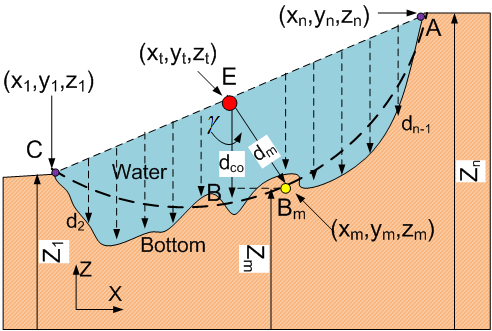 | Figure 9. Sketch definition of mean depth at critical overflow |
The point E: | (29) |
The point Bm: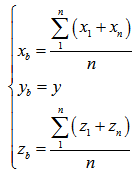 | (30) |
On the basis of equation (29) and (30), it is not difficult to find the desired parameters through the following equations. | (31) |
Where the subscript m, t and b denotes mean, top and bottom respectively. | (32) |
And | (33) |
Another approach to find out dco is using equation(20). In fact, angle γ is a very small and approach to zero. Once the horizontal position of the point B is decided, the corresponding elevation of DEM for the point B is also confirmed by combining it with the known spatial location of point B in longitudinal direction (thus y direction). This is because the calculation is based on DEM through.At this stage, the formulas and their parameters applied in cross-sectional direction are already obtained.In the following subsections, the concentration is to be located on longitudinal direction along flood channel.Bed Slope and Curvilinear Length Both bed slop (S0) and curvlinear length(s) are scales to discribe how fast the quantity of parameter such as specific engery and kinetic energy varies along longitudinal channel. In flooding, the bottom of channel could be more irregular than that of natural channel. The bed slope is able to be gained by finding mean values of elevation like the manner of handling parameters at one cross section. Figure 10 shows a general case that the fluid flows in a very rough channel. Assume that there are two arbitary sections: section 1 and 2. 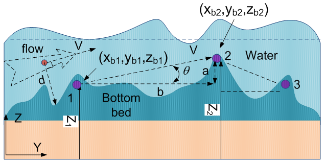 | Figure 10. Side view of flood over bottom of flood channel |
The bed slope(S0) and their spatial distance (s) are determined by following up the direction of flow. Although both velocity at point 1 and 2 are vector and many velocity points on stream lines between two sections can be selected, the most convinent and effective manner is to chose the mean value for them at the bottom (see Figure 11).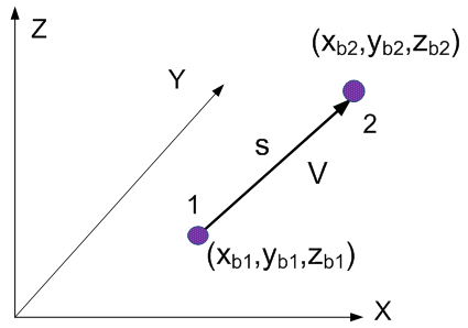 | Figure 11. sketch definition of curvilinear length |
Assume that there is a triangle between section 1 and 2 in Figure 10, where a and b respresent vertical height and horizonal distance, and θ is the slope angle. Then, the spatial relation can be easily confirmed by the following equations. | (34) |
Where  Then, curvilinear length S between two arbitry sections is gined by the following equation.
 | (35) |
Friction Slope, Bed Slope and Depth VariationThere are two slopes which are often used in hydraulic engineering.The friction slope (Sf) is to describe how kinetic energy varies when flow travels in channel. It is defined as follows. | (36) |
In pratice, on the basis of equation (13) or (14) and equation (35), it can be numerically treated as | (37) |
For any arbitary cross sections.Bed slope (S0) is defined as (see Figure 4) | (38) |
The slope angle (θ) is determined by equation (34).The variation of the depth of flow with logitudinal distance in a channel with arbitrary shape [13] is discribed by the following equation. | (39) |
Where, Fr , Sf , and S0 is determined by equation(12),(37) and (38) respectively.At this stage, some necessary concepts used in modelling are already reviewed and introduced. Because the modelling is to be performed based on information supplied by both remote sensing imagery and DEM. In the following subsections, the focus is to be positioned on how to extract useful data and applied them into modelling flood intergrating them with the knowledge of hydraulic engineering.
3.2. Utilization of Remote Sensing Imagery and DEM
There are a lot of useful imformation stored in remote sensing imagery and corresponding DEM. To gain them, Of importance is to uderstand that1) the correlation between remote sensing imagery and DEM, and how they are formed respectively at technical level. 2) How the digital image and DEM is processed respectively.Characteristic Absorption Band of Observed SubstancesSome substances such as water and vegetation captured and stored by remote sensing imagery are easily distinguished according to the characteristic absorption band (see Figure 12). The supplied information is very useful to sample desired substance from remote sensing imagery. Its application is to be introduced in the subsections. 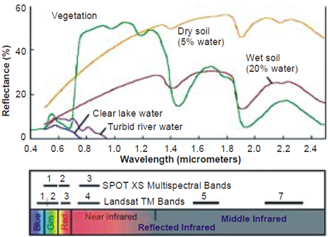 | Figure 12. Characteristic absorption band of observed substances [18] |
Correlation between Remote Sensing Imagery and DEMAlthough observed objects can be delicately identified by norrow bands (continuous), such approach is powerful to verify fine components of substances. Its principle is similar to the ones supplied in analytical chemistry. For the digital image of landscapes such as imagery of LANDSAT, its bands are discontinuous. However, from the angle of engineering applications, it may be accurate enough to apply extracted data and information into practice. To do so, of importance is how to establish the correlation between remote sensing imagery and DEM so that individual information can be mutaully and accurately transferred, displayed and then fully utilized in further developments.Figure 13 illustrates the basic concepts of romte sensing imagery and DEM. In mathmatics, both of them are formed by means of a matrix which has specified dimensions for each of them respectively. Each row and column is indicated by the corresponding a unique paire of indeces (j,i).In the digital image processing, there are many techniques in idenfying captured objects, however the basic colours are Red, Green and Blue. Therefore, identifying investigated objects on the surface of the Earth can be handled by means of their pixel locations and their intensities, thus digital numbers. 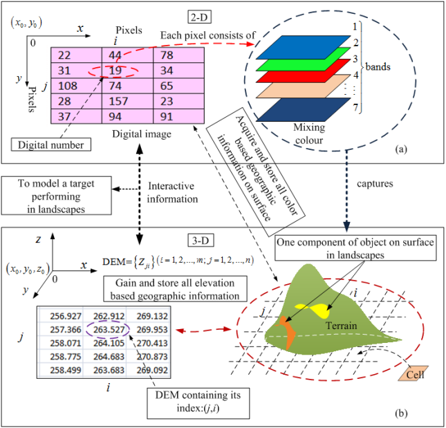 | Figure 13. Correlation between remote sensing imagery and DEM |
On the other hand, there are several geometric parameters of discribing terrain such as slope,aspect , profile curvature, plan curvature and roughness, those values can be obtained from DEM. Their definitions and applications can be found from useful references [19-21]. Finally, the individully extracted information and data from remote sensing imary and DEM can be accurately transferred and displayed in different systems (thus Cartesian coordinates) on demand using the technique of linear indexing as its backbone. The linear indices are generated by the corresponding row and coloumn index (j,i) in the matrix. However, the precondition to mutally transfer data and information is that both of remote sensing and DEM must has the same dimensions. Otherwise, this approach is impossible to carry out.An Exsample to Demonstrate To demonstrate above procedure, an example is supplied as follows.Figure 14 is a romate sensing imagery capatured by LANDSAT 7.4.2, its geographical site is shown in the following box. The corresponding DEM (SRTM3 offered by USGS) is displayed in Figure 15. In this case, assume that the river is an object to be investigated. Applying above procedure into the imagery, the river is easily detected in remote sensing imagery because water is a pure substance in comparison with other objects such as vegetation and soil (see Figure 12, Figure 14 and Figure 16). Of course, during this approach, there is one important step—sampling, which is to be introduced in the following subsection. 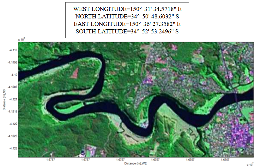 | Figure 14. River is shown in remote sensing imagery (349×674) captured by LANDSAT 7.4.2 |
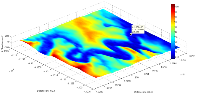 | Figure 15. DEM (349×674) corresponding to its remote sensing imagery |
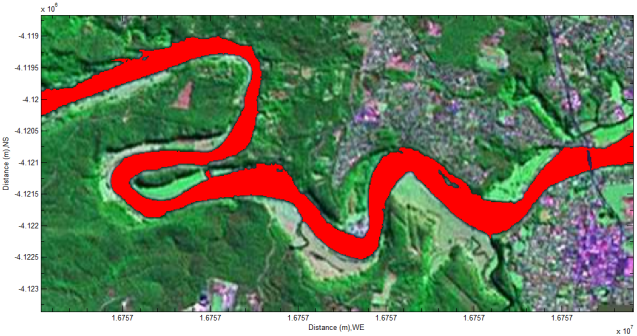 | Figure 16. Detected river (red color) remote sensing imagery captured by LANDSAT 7.4.2 |
Display Gained Information into DEMThe next step is to transfer gained information thus data of river from Figure 16 into the corresponding DEM (SRTM3 offered by USGS) in Figure 15. In order to clearly visualize and verify the detected river shown in the DEM, the elevation of the detected river is increased by adding 20 meters to the original elevation of river before it is displayed into DEM (see Figure 17). 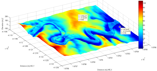 | Figure 17. Detected river shown by DEM |
Build Coordinates Using Convention of DEMAnother noticed topic is related to the difference between the eleveation of DEM (H) and depth of river, lake and flood channel (d). In this research, the vertical height (elevation) of lake and flood channel is measured on the basis of the convention of DEM (see Figure 18). The coordinates (X-Y-Z-0) is built on the horizontal sea level. The depth of lake or flood channel (d) may be equal to the elevation of DEM at the sea level in the specific case. 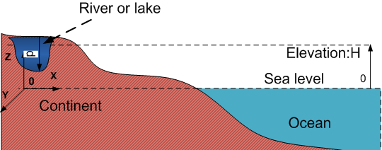 | Figure 18. Elevation of river or lake and convention of DEM |
Determine Elevation and Depth of Lake or RiverThe depth of lake and river is a variable. In the most cases, it varies with time, flow rate and so on. In other words, the elevation of water front is important parameter to determine the depth of lake and river. Although the information about water front supplied by remote sensing imagery is static (see Figure 19), its track of flow is an important proof to not only identify and classify water and bank but also forecast the risk of local area to be inundated. 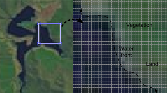 | Figure 19. Water front displayed in remote sensing imagery |
To effectively classify the boundary of water and land, one of important steps is sampling. Although the process of classifying substances in the remote sensing imagery can be automatically implemented by building computer codes, the location of pixel and selected value of R, G and B affect the quality of classifying substances. In general, the sampling always takes place in the middle of lake or river because the pixel of water in the middle of lake or river is not much affected by other substance such as vegetation (see Figure 20) in comparison with pure water shown in Figure 12. 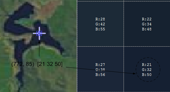 | Figure 20. Sampling water in lake shown by remote sensing imagery |
Once the lake or river is succesfully detected, the elevation of water front thus the maximum elevation of DEM near the water front is confirmed. At the same time, the maximum depth of lake or river, thus the distance from the water surface to the minmum elevation of DEM at the bottom of lake or river within the area of lake or river can also be determined. The elevation of water front is an important value to be used in further approach to model flood.Determine Possible Inundated Area Discovering which area to be inundated is a very important step. The snificance appears in not only effectively modelling flood but also the natural desarster control and management.There are two steps to perform this approach.1) Find a local lake from Figure 1 and handled it using the above manners. The detected lake (blue colour) is then shown in Figure 21. In this case, the maximum elevation of detected lake thus water front is 308.05 meters. This value is used to detect potential zones to be inundated if storm occurs in this area. 2) Set the condition like 308.05 meters <= elevation of landscape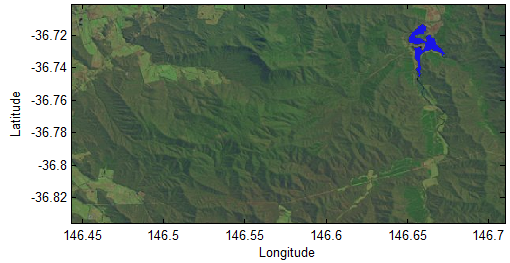 | Figure 21. Detected lake in satellite imagery |
Then the possible inundated zones are easily detected.Because the detected risk zones are indexed (in the same matrix), they can be displayed in both remote sensing imagery and the corresponding DEM (SRTM3 offered by USGS) (see Figure 22 and Figure 23) using above technique. As mentioned above, in order to clearly visualize the detected risk zones in DEM, the elevation of them displayed in Figure 23 is increased by adding 200 meters to the original elevation. | Figure 17. Detected river shown by DEM |
Display Interested Section of Risk ChannelFor one certain purpose, any elevation of risk zones shown by Figure 22 and Figure 23 can be analysed and utilized further by arbitarily selecting one desired area. To do so, the interested area can be easily selected by using brush functionality in MATLAB®. The data is then plotted in two-dimension (see Figure 24). 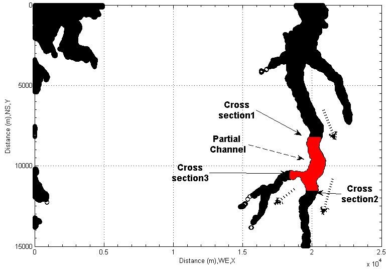 | Figure 24. Select partial channel from one of possible inundated areas |
Above procedure, in fact, is one step to find out the relevant linear indices of the selected area by means of obtained spatial location and their spatial vector conversion. Once the linear indices are confirmed, the partial area thus the interested area can be displayed by three-dimension(see Figure 25) because this process happens within the same matrix.Above procedures demonstrate how to detect possible inundated area by means of finding the local lake, and then find the interested area to focus on by using the maximum elevation of local lake as a criterion and arbitrarily selecting desired zone. However, this is not a final approach for this research. The target of this research is to model flood. The further approach is to perform in the following subsections.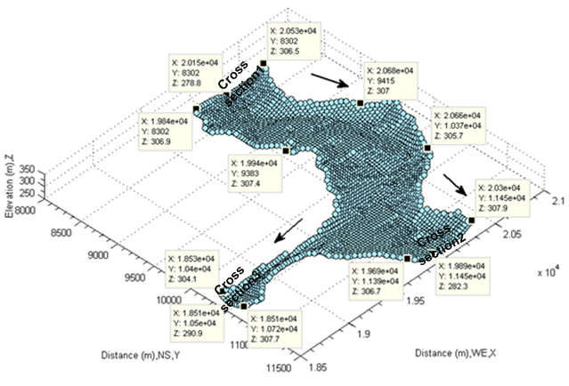 | Figure 25. Displays partial channel in three-dimensional coordinates |
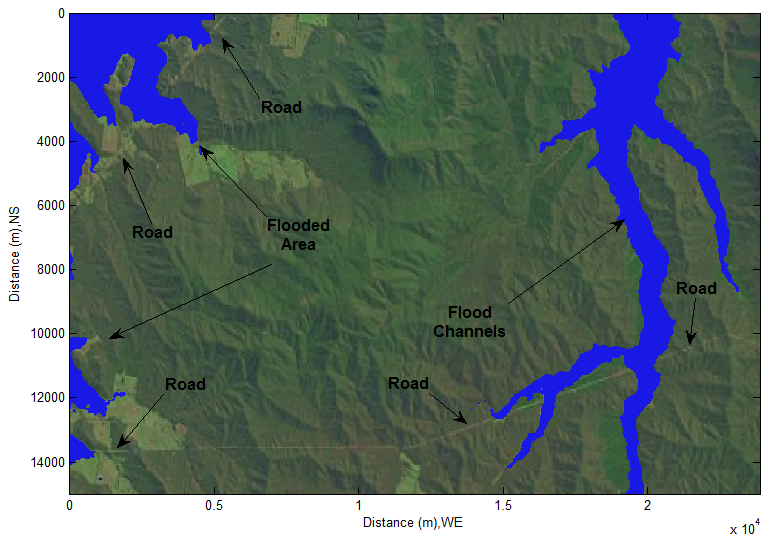 | Figure 26. Discovered flood areas in the remote sensing imagery |
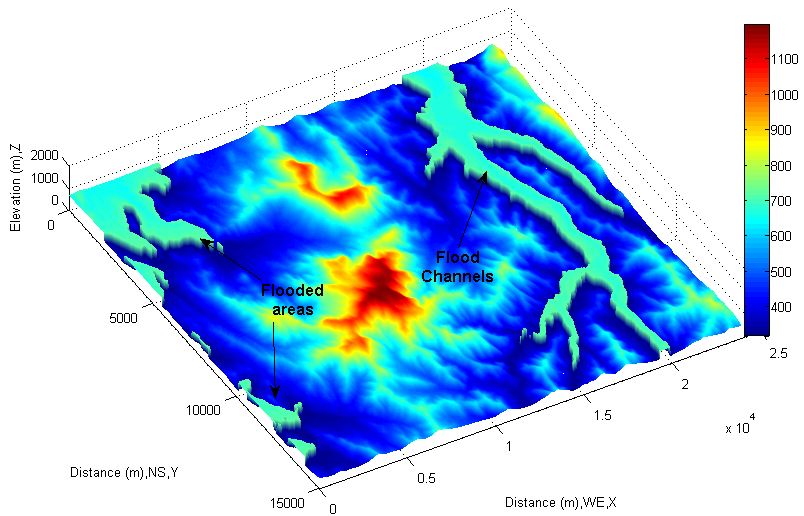 | Figure 27. Display flood areas in DEM |
Determine Flood Area In fact, determining flood area is not so difficult based on above discoveries. Only one task to do is altering the existing hydraulic criterion. If the area whose elevation is equal to or less than the elevation of water surface of lake plus one certain height is decided, the possible level of flood is then confirmed. The certain height indicates the level which flood could rise to. In this case, assume that the maximum height which flood water could rise to be 10 meters, then the modified algorithm becomes as follows.308.05 meters +10 meters <= elevation of landscapeFollowing up the same procedures introduced above, the possible flooded areas are easily detected. Similarly, the updated area is displayed into original remote sensing imagery and corresponding DEM (see Figure 26 and Figure 27) respectively.The difference after rising elevation of water surface is easily found by comparing the flooded areas in Figure 26 with the possible inundated areas in Figure 22.In some areas, areas are enlarged and lengths are extended. Very clear, it is caused by raising the elevation of water surface in those areas. The attention to which should be paid is the mathematical sign “<=”. The physical meaning confines and indicates how much the elevation of water surface possibly rises to during flood. In terms of the existing trace recorded in the remote sensing imagery, the flooded zones controlled by the sign “<=” are consistent with the real cases. Accordingly, the extracted information is very reliable.At this stage, the pre-conditions of modelling flood in this area are already built.Choose Desired Area to Model FloodThen, repeat above procedures to choose desired area (see Figure 28 and Figure 29) to model flood. 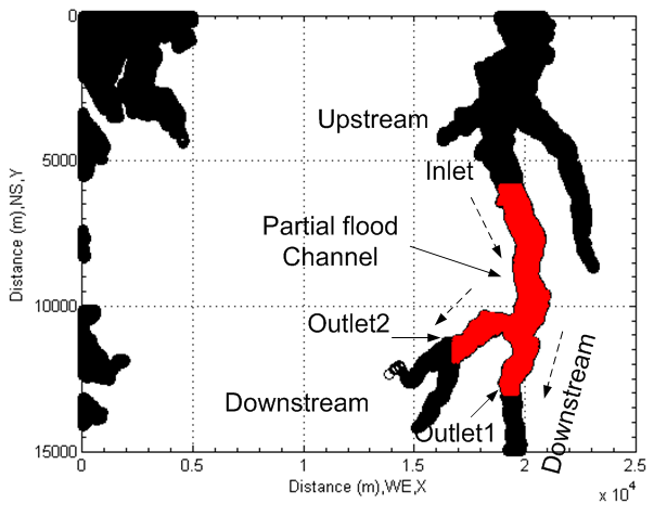 | Figure 28. Select arbitrary flood channel for modeling |
 | Figure 29. Insert selected flood channel into original remote sensing imagery |
Up to this point, some necessary pre-preparation of modelling flood in specified area is already made. In the following subsections, the approach is to discuss how to further select desired data for calculation using specific knowledge in hydraulic engineering.
3.3. Geometric Feature of Selected Flood Channel
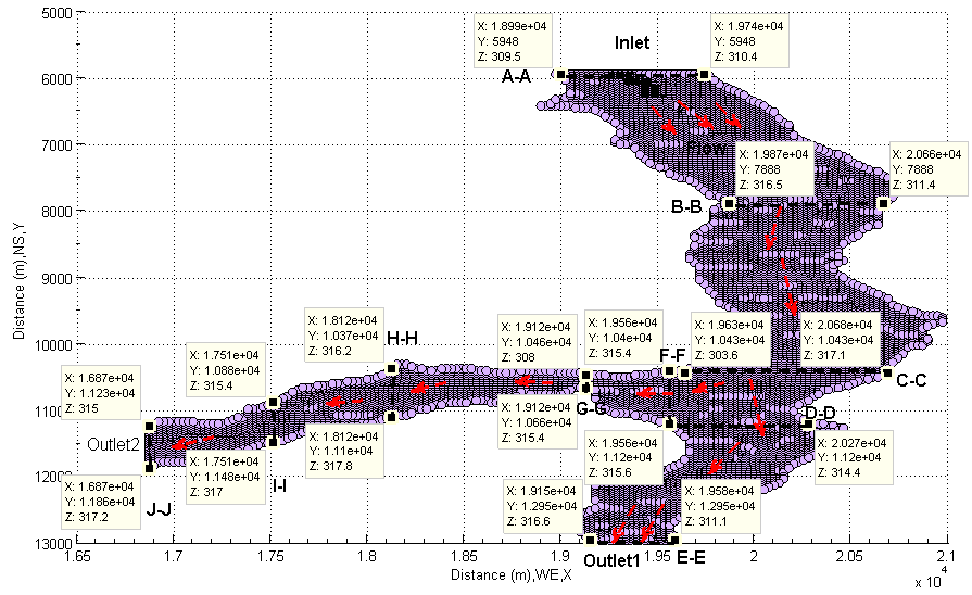
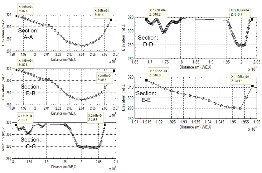
Following up above procedures, the selected flood channel shown in Figure 28 and Figure 29 is then transferred within the same matrix by using the discovered linear indices. Its three-dimensional terrain is separately shown in Figure 30. The corresponding flood channel of top view is represented in Figure 31.In order to investigate hydraulic characters of flood in detail, several cross sections (from A-A to J-J) are arbitrarily selected (see Figure 31). Then, the corresponding cross sections are represented in Figure 32 and Figure 33. Those cross sectional channels are very irregular when flood happens in this area. The traditional manner of calculating cross sectional area may be difficult to handle such complex cases. Fortunately, MATLAB® provides the calculation with a built-in function: ployarea. This built-in function is created by the theory of computational geometry. All points on those cross sections become two group arrays in different direction. Hence, the pair of X and Z represents a series of spatial points (thus ,vectors in a matrix) at each cross section along longitudinal direction respectively, the pair of Y and Z represents vectors at each cross section along transversal direction. Applying sampled data into this built-in function, each cross sectional area is then generated. However, the attention to which should be drawn is that 1) Most of those channels does not have the exact horizontal surface because the mathematical sign “<=” is used to forecast how flood water rises from the bottom of flood channel and then estimate how much big the cross sectional area is when the overflow happens at both side of channel bank. The detailed discussion is already performed in preceding sections (see Figure 6 and Figure 7).2) The calculated cross sectional area is the area when overflow or floodplain starts to take place from both sides. In other words, the concept can be also extended to any cross sections along flood channel. Thus, it is a critical cross sectional area for any cross sections along flood channel when the flow rate or velocity of flow reaches to a critical value and water overflows from both side of flood channel bank. 3) It is not a cross sectional area for the case that water overflows from single side, thus the low elevation side of flood channel section because the flow rate is not large enough or the speed of water is slow when water passes the cross section. In other words, if the flow rate (Q) is not large enough, it may not cause floodplain. However, in the process of modelling flood, the mathematical sign “<=” covers all areas where meet the selected criterion (thus 318.05 meters). The less attention is paid to the process of how the flood rises from the bottom of flood channel in this research. 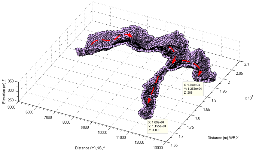 | Figure 30. Display selected partial flood channel in three-dimensional coordinates |
 | Figure 31. Top view of flood channel with selected cross sections |
 | Figure 32. Longitudinal cross sections in flood channel |
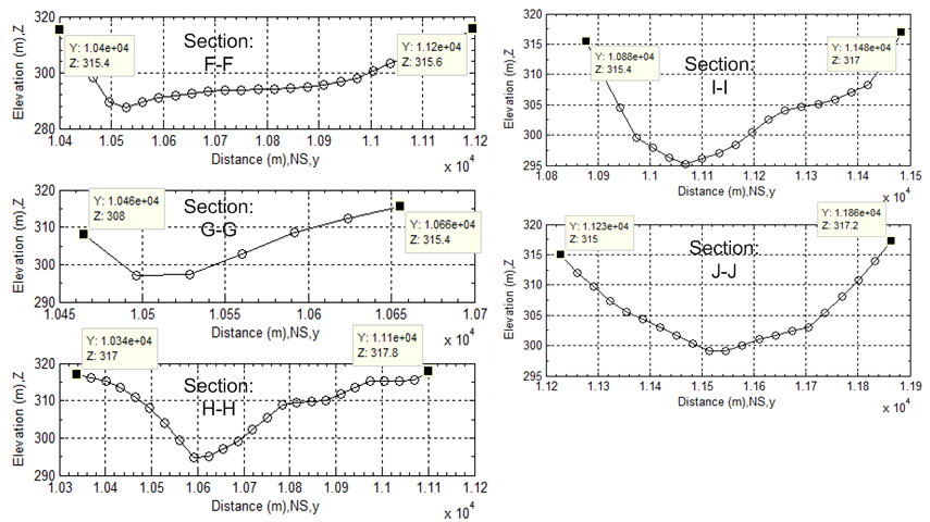 | Figure 33. Transversal cross sections in flood channel |
3.4. Classification of Channel Flow
Figure 30 provides not only geometric features of flood channel but also useful information to assess how flood flow is disturbed by irregular shapes of channel. According to the definition of Reynolds number, | (40) |
Where V is characteristic velocity flow, in hydraulic engineering it is often replaced by mean velocity of flow.μ is kinetic viscosity of fluid at specific temperature and pressure.L is characteristic length, in hydraulic engineering it can be assessed by using the hydralic radius(Rh). Reynolds number is dimensionless number; the type of flow can be classified as follows. In this research, the dynamic viscosity of water, μ =7.97e-4 Pa∙s at pressure 1e+5 Pa and temperture 303 K is selected respectively.In reality, the most type of flow is turbulent flow. The transitional flow lies between laminear flow layer and turbulent flow layer. In flooding, the turbulent flow often appears at two layers. One is top surface layer. In this layer, wave travels in manner of forward and backward style. Another happens at layer of channel bottom. In the bottom layer, turbulent flow is caused by roughness. Figure 34 is longitudinal profile of flood channel. In terms of information of the elevation of water surface in lake, the surface layer over 308.05 meters thus the line CD belongs to turbulent layer. Thus the square ABCD is turbulent layer. The triangle FEG consists of turbulent layer too at bottom of flood channel. The square DCEF lies in the middle layer, it may belong to the transitional layer. Similarly, the turbulent and transitional layer can be found in Figure 35 as well.On the other hand, there is a slope which can be found in both Figure 34 and Figure 35 respectively. The slope angle (∅ and α) in longitudinal and transversal direction respectively is approximately equal to 0.2°.
 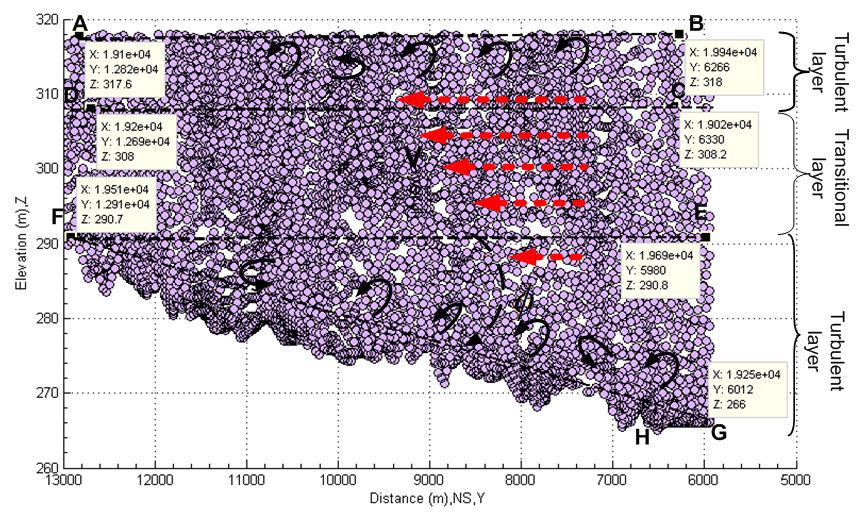 | Figure 34. Longitudinal view of flood channel |
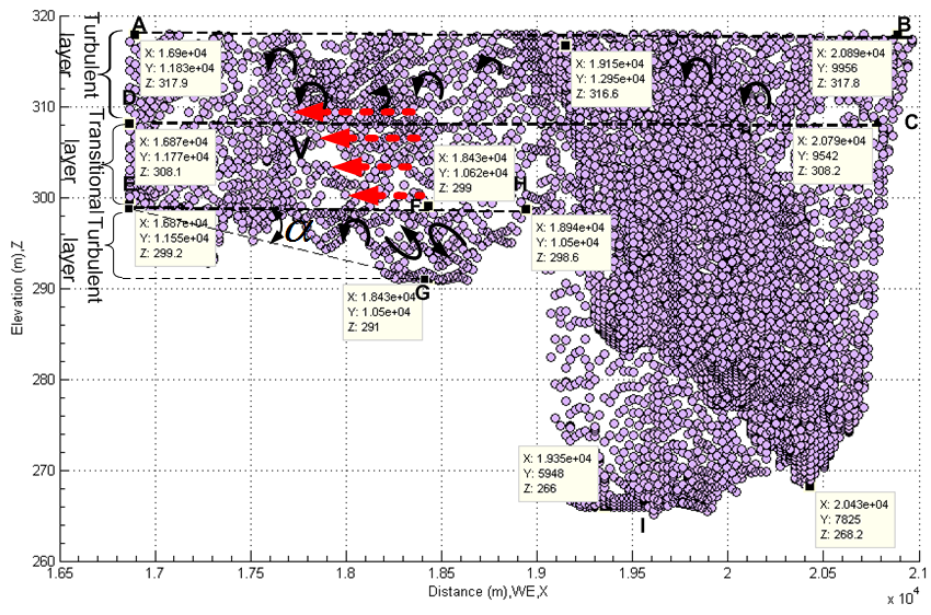 | Figure 35. Transversal view of flood channel |
4. Results and Discussion
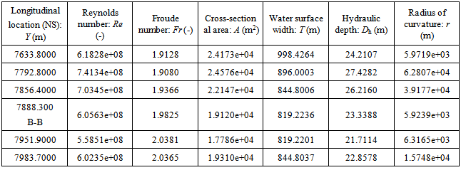
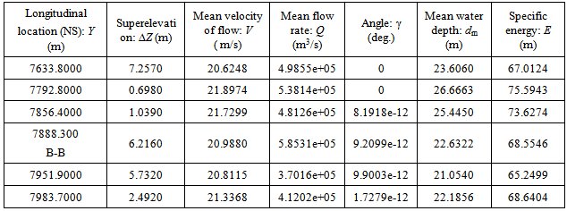
The results are generated by the calculation using the extracted data from remote sensing imagery and corresponding DEM and formulas developed by the new concepts for modelling flow in the critical state of overflow, thus in the state of hazard. The results are classified into three types. The first results in Table 1 to Table 6 are yielded on the basis of selected cross section shown in Figure 31 to Figure 33 to focuse on analysis of some main hydraulic parameters. The second results in Table 7 to Table 9 provide more detailed information about flood flow at the cross sections close to the section B-B. Eventually, the longitudinal velocity distributes in transervsal direction is discussed. Some relevant results (from Figure 37 to Figure 39) are also supplied.
4.1. Common Hydraulic Properties at Each Selected Cross Section
On the basis of information supplied in Table 1 to Table 6, it can be discovered that1) According to Reynolds number (Re) and Froude number (Fr) in Table 1, it is easily to identify that flood passing through whole selected cross sections with one mean velocity belongs to the turbulent flow. When overflow at both side banks happens, the flow is in a supercritical state and the inertial forces are dominant because of Fr>1(see Figure 3). Reynolds number (Re) and Froude number (Fr) is calculated by equation (40) and (12) respectively. In this case, the slope angle (θ) used to calculate Froude number (Fr) and the celerity of wave(C) using equation (15) is 0.2°. kinetic energy correction factor ζ equals 2.0 because water overflows from the both side bank and the flow has very fast speed. However, in terms of the data listed in the subsection, the slope angle is a sensitive parameter for some hydraulic parameters such as specific energy. In the first group of data except for Froude number (Fr) and the celerity of wave(C), the rest parameters do not have a direct relation with the slope angle.2) Table 2 to Table 4 provide some geometric values of flood channels. As seen from Figure 32 and Figure 33, the flood channel is usually very irregular. Those values including ones in Table 5 are calculated by equation (1), (2), (5), (12), (15), (19), (20), (21) and (23) respectively. 3) The superelevation (∆Z) listed in Table 4 is difference between the maximum and minimum elevation at both side banks. They vary at all time along longitudinal direction of channel. As seen, such difference exists in all cross sections because this is a typical natural geometric feature. Relying on such a feature, it is easier to find its corresponding curvature radius. Actually, such as concept can be extended to any level of flood during the period of water rising from the bottom of flood channel. The critical overflow is only a special case.4) In the process of calculating longitudinal critical overflow velocity (Vco) using equation (23), the flow rising parameter (ω) is set as one because the transversal distribution of velocity (Vco) is not taken into account. Thus it is treated as a mean velocity. According to the continuity of fluid, the result of calculation using such a treatment may not cause too much error. The detailed discussion about its transversal distribution is to be performed in the last subsection.5) Furthermore, in terms of information offered by Table 5 to Table 6, it can be concluded that the scale of flood could be very large at range of elevation between 308.05 and 318.05 meters.6) Because Fr>1 and the mean velocity of longitudinal flow is larger than the celerity of wave, thus V > C, it can be concluded that such a flow is in subcritical state, the wave cannot propagate upstream against the flow, and upstream areas are not in hydraulic communication with the downstream areas.Table 1. Reynolds and Froude number in longitudinal and transversal flood channel
 |
| |
|
Table 2. Cross sectional area and wetted perimeter in longitudinal and transversal flood channel
 |
| |
|
Table 3. Water surface width and hydraulic radius in longitudinal and transversal flood channel
 |
| |
|
Table 4. Hydraulic depth and superelevation in longitudinal and transversal flood channel
 |
| |
|
Table 5. Radius of curvature and mean velocity in longitudinal and transversal flood channel
 |
| |
|
Table 6. Mean flow rate and celerity of wave in longitudinal and transversal flood channel
 |
| |
|
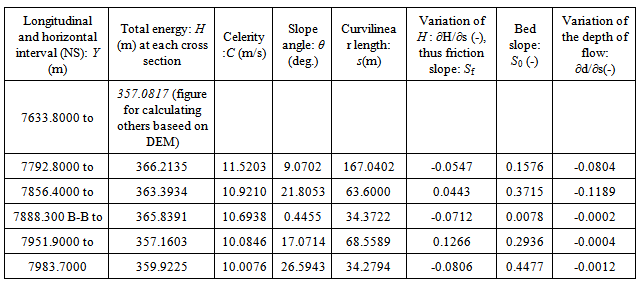
4.2. Detailed Hydraulic Properties
Relying on the results shown in the last subsection and information gained from cross sections neighbouring to the cross section B-B, it is easily found that flood is in the turbulent and subcritical state when the critical overflow occurs. Except for the equations indicated in the last section, extra equations are used in this section. The angle (γ) , mean water depth (dm), specific energy (E), total energy (H), slope angle (θ), curvilinear length(s), friction slope(Sf), bed slope(S0) and depth variation is calculated by equation (32),(31),(4),(34),(14),(35),(37),(38) and (39) respectively. The main difference between calculations is that the slope angle (θ) used in the later calculation is measured and calculated by using local curvilinear length(s). The later approach dramatically improves the accurateness of calculation because the sampled interval between two cross sections becomes smaller. In terms of information from Table 7 to Table 9 and Figure 36, it can be found that 1) The longitudinal distribution of friction slope and depth variation is sensitively affected by the variation of slope angle (θ) respectively and varies along longitudinal curvilinear length with respect to time.2) However, the celerity (C) of wave approaches to the decreasing state. That is because Fr>1 and the mean velocity of flow is larger than the celerity of wave, thus V > C. 3) Another interesting discovery is that angle (γ) (see Figure 9) approach to zero. That indicates that the radius normal to the bottom can be directly replaced by the vertical radius of flow in the critical overflow state, thus the elevation of water surface at each point on width (T) can be directly used for hydraulic energy calculation.In the preceding two sections, the most common hydraulic parameters are already illustrated and discussed when the flow passes each cross section in the critical state of overflow with one mean speed. However, the average velocity of flow fails to describe how the flow passes through the cross section in detail. Accordingly, in the last subsection, the attention is to be drawn to discuss how the longitudinal velocity distributes in the transversal direction at any cross section along the flood channel.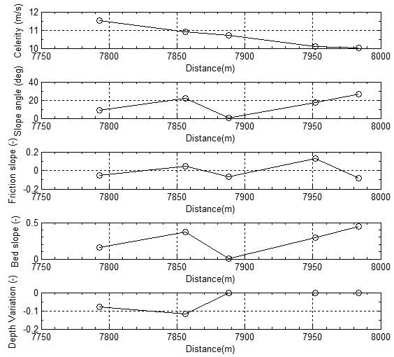 | Figure 36. Celerity, slope angle, friction slope, bed slope and depth of water vary with longitudinal distance in flood channel |
Table 7. Hydraulic and dynamic properties of flow and fluid adjacent to cross section B-B in longitudinal flood channel
 |
| |
|
Table 8. Hydraulic and dynamic properties of flow and fluid adjacent to cross section B-B in longitudinal flood channel (continued)
 |
| |
|
Table 9. Bed slope, variation of kinetic energy and depth of water flow with longitudinal curvilinear length adjacent to cross section B-B in longitudinal flood channel
 |
| |
|
4.3. Discover Distribution of Longitudinal Velocity in Transversal Direction
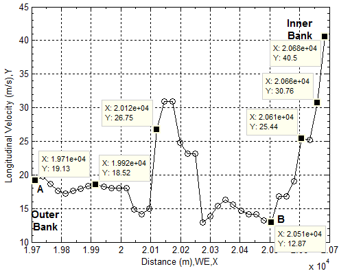
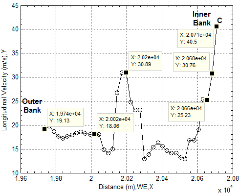
In the last two subsections, the average velocity of flow is already used to calculate other values of hydraulic parameters. In general, it is fine for most hydraulic applications. However, in practice, the more interesting sometimes is positioned onto the distribution of flow velocity in transversal direction. In order to illustrate and explore this process, the cross section locating at Y= 7633.8000 meter (see Table 8) is chosen to further investigate the hydraulic properties of flow at the cross section. Figure 37 offers the elevation of flood channel bottom at this section. Figure 38 and Figure 39 provide the distribution of longitudinal velocity across the selected cross section of flood channel. Each longitudinal velocity at each subsection on the wetted perimeter (Pw) is calculated by using equation (23) and (24). The used data are extracted from remote sensing imagery and DEM respectively. There are several key points or steps which should be taken care of when equation (23) and (24) are used.1) In the first approach, the flow rising parameter (ω) is set as 1.0 when equation (23) is used, this figure is treated as a trial value for the specific case of critical overflow.2) Apply the partitioned water surface width corresponding to the subsection of the wetted perimeter at the bottom of flood channel into equation (23) and set the value of the conversion coefficient k to be 0.1 to calculate longitudinal velocity along transversal direction, and then the longitudinal velocity distribution in the transversal direction, average velocity located in subsections is obtained respectively.3) Verify above obtained data in comparison with the mean longitudinal velocity (20.6248 m/s, see Table 8) calculated by equation (23) setting ω=1.0.In this case, the average longitudinal velocity in the transversal direction is 18.9573 m/s when k is assigned as 0.1. It is very close to already obtained mean velocity. The error between two values of mean longitudinal velocities (thus, 20.6248 m/s and 18.9573 m/s) is caused by the counted number of subsections (see Figure 8). Because the length of one subsection is formed by two spatial points, in the matrix operation, the multiplication between two vectors must have the same dimensions. Therefore, in the first calculation, the first to (n-1)th subsection is considered (see Figure 38); in the second calculation, the second to nth subsection is used (see Figure 39). Accordingly, in fact, no error exists if two separately calculated data are located together (see the spatial point A, B and C in Figure 37, Figure 38 and Figure 39 respectively).4) Then the value of flow rising parameter ω=1.0 and conversion coefficient k =0.1 in this trial is confirmed respectively.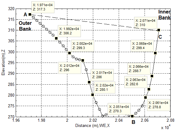 | Figure 37. Elevations of bottom surfaces distribute across flood channel |
 | Figure 38. Longitudinal velocities distribute across flood channel section (a) |
 | Figure 39. Longitudinal velocities distribute across flood channel section (b) |
In the case of critical overflow, it can be obviously discovered that 1) The longitudinal velocity at the inner bank is larger than the one distributing along the outer bank. This phenomenon is completely consistent with the real case as well as “the water depth increases from the inner bank to the outer bank while the depth-averaged velocity is maximum at the inner bank. In practice, flow resistance affects the velocity field but maximum velocity is observed towards the inner bank” , which is described by Chanson [14] by means of the theoretical derivation and other reports. 2) The transversal distribution of the longitudinal velocity is seriously affected by the shape of the bottom of flood channel. In general, the velocity close to the inner bank is larger than that at the outer bank. However, the distribution of longitudinal velocity at both side banks is directly affected by the slope angle of bank wall. The velocity close to the steep wall is larger than that having larger slope angle.3) The longitudinal velocity at the minimum depth such as point B (see Figure 37 and Figure 38) has less influence from obstacles. Therefore, the roughness is mainly created by the sloped substances at the bottom of flood channel.Further consideration abut Discoveries Using DEMAs noticed from above discoveries, the value of the conversion coefficient k equals 0.1 actually uncovers and indicates the following hidden topics those are required to further consider.1) The shape of cross section is not taken into account when the mean longitudinal velocity is calculated by using equation (23) and assuming ω = 1.0 as the critical overflow. 2) Above treatment, in fact, is a manner of that● The mass center in fluid volume at the cross section is treated as a firmed spatial point locating in the central line in open channel (see equation (18) and Figure 5). Hence, the flow is treated as the uniform along the longitudinal flood channel.● The complicated terrain locating at the bottom of flood channel is ignored. Thus, the effect of resistance at the bottom of flood channel is neglected. Such an effect is also termed as the roughness. Manning’s resistance coefficient n used in equation (16) was introduced for this purpose and the target of equation (17) is to seek for a reliable n, but the problem is that there is a condition to use this equation. Furthermore, to assess whether the flow in newly selected open channel meets this condition or not, other measurements are required. Therefore, the process could be very complex. In the new approach, the roughness can be already included into the conversion coefficient k. The experiments of determining roughness are not necessary to carry out.● The longitudinal velocity evenly distributes in transversal direction. Although several historical research results in this field were collected [12]. However, the supplied equations have similar drawbacks; hence they have to rely on many other parameters whose values are usually unknown before they can be applied into specific cases. Very clear, above factors cause a lot of errors and difficulties to use the supplied equations.In the new approach, in order to meet the principle of fluid continuity, the value of the conversion coefficient k in most natural channels must be less than one to compensate for the above ignored factors. This approach is already mentioned in equation (27) and (28). A practicable case is therefore supplied to demonstrate. Based on above understanding, the application can be further extended to the general cases, hence the cases those the values of ω are chosen at the range of 0≤ω(t)≤1. Consider the process of the increasing magnitude of longitudinal velocity is complicated, accordingly two equations to describe it are proposed and already discussed in the preceding section (see equation (25) and (26)). Once the value of ω at the specified time (t) is given, above technique is still useful to calculate the values of desired hydraulic parameters. However, the approach is limited to seeking for similar flow rate and average velocity by arbitrarily adjusting the location of starting subsection of wetted perimeter and the length of it. Then, the real elevation of water in the flood channel can be forecasted in such a manner.
5. Conclusions
This research is different from other style of modelling flood. It is an interdisciplinary research focusing on an application in hydraulic engineering, thus modelling flood. The new approach has the following features. 1. The topographical data of flood channel was extracted from remote sensing imagery and the corresponding digital elevation model.2. In order to demonstrate the procedure. Some necessary principles and concepts about how to integrate remote sensing imagery and the corresponding DEM have been introduced. On the basis of this composited technique, the spatial location of lake or river can be easily detected in the remote sensing imagery and its data and information can be accurately transferred into DEM. On the other hand, the advantage of DEM is also discovered and utilized. Such united advantage provides a powerful backbone in modelling flood.3. In the process of modelling flood, in order to discover the local zones to be inundated and how flood is performed. An easy and accurate manner has been discovered by selecting the elevation level of local lake as a criterion. The detected zones are consistent with the ones used to be flooded and stored into remote sensing imagery. This approach also has significant meaning in forecasting and controlling large scale flood.4. Then, the data of selected flood channel can be accurately transferred into DEM as an investigated object to model.5. The further modelling was performed on each arbitrarily selected cross section. Those cross sections show very irregular. 6. The average longitudinal velocity of flow in the flood channel can be calculated by the modified equation by means of the curvature radius and superelevation at any arbitrary cross sections of flood channel. Both curvature radius and superelevation actually is the natural topographic feature for each cross section. The values of them can be easily gained in the DEM based process. In other words, the mean longitudinal velocity can be also regarded as a natural feature for any cross section in the natural pen channel. 7. Due to such a unique feature, the flow rising parameter was introduced to describe how the magnitude of longitudinal velocity increases when water rises from the bottom of flood channel. And also assume that longitudinal velocity is a critical overflow speed when the value of the flow rising parameter is set as one. This treatment simplifies the process of calculation and avoids directly considering the complicated shape at the bottom of flood channel. 8. Based on above approaches and the convention of terms, some values of important hydraulic parameters can be easily achieved. 9. In order to know how the longitudinal velocity distributes in the transversal direction at any arbitrary cross section, a conversion coefficient was introduced. On the basis of continuity of flow, the conversion coefficient is able to not only transfer data but also provide information about several hidden and ignored factors. 10. All calculated data can be easily and accurately displayed in each process. In short, modelling flood is one part of applications in hydraulic engineering by means of accurately and effectively integrating remote sensing imagery and DEM. The research in further applications is in progress.
ACKNOWLEDGEMENTS
Author wants to offer special thanks to Professor Jing. X. Zhao at Shanghai Jiao Tong University for supplying desired data used in this research.
References
| [1] | Damle, C. and A. Yalcin, Flood prediction using Time Series Data Mining. Journal of Hydrology, 2007. 333(2-4): p. 305-316. |
| [2] | Degiorgis, M., et al., Classifiers for the detection of flood-prone areas using remote sensed elevation data. Journal of Hydrology. 470–471: p. 302-315. |
| [3] | Hostache, R., et al., Water Level Estimation and Reduction of Hydraulic Model Calibration Uncertainties Using Satellite SAR Images of Floods. IEEE Transactions on Geoscience & Remote Sensing, 2009. 47(2): p. 431-441. |
| [4] | Tarekegn, T.H., et al., Assessment of an ASTER-generated DEM for 2D hydrodynamic flood modeling. International Journal of Applied Earth Observation and Geoinformation. 12(6): p. 457-465. |
| [5] | Yamazaki, D., et al., Adjustment of a spaceborne DEM for use in floodplain hydrodynamic modeling. Journal of Hydrology. 436–437(0): p. 81-91. |
| [6] | Ballesteros, J.A., et al., Calibration of floodplain roughness and estimation of flood discharge based on tree-ring evidence and hydraulic modelling. Journal of Hydrology. 403: p. 103-115. |
| [7] | Blomgren, S., A digital elevation model for estimating flooding scenarios at the Falsterbo Peninsula. Environmental Modelling and Software, 1999. 14(6): p. 579-587. |
| [8] | Cobby, D.M., D.C. Mason, and I.J. Davenport, Image processing of airborne scanning laser altimetry data for improved river flood modelling. ISPRS Journal of Photogrammetry and Remote Sensing, 2001. 56(2): p. 121-138. |
| [9] | Fewtrell, T.J., et al., Benchmarking urban flood models of varying complexity and scale using high resolution terrestrial LiDAR data. Physics and Chemistry of the Earth, Parts A/B/C. 36: p. 281-291. |
| [10] | Yangbo Chen, K.T., Ian Cluckie & F.Hilaire De Smedt, ed. Gis And Remote Sensing In Hydrology, Water Resources And Environment. 2012, IAHS Press: France. |
| [11] | Center, U.A.C.o.E.I.f.W.R.H.E. (2008) HEC-RAS River Analysis System User’s Manual. |
| [12] | French, R.H., Open Channel Hydraulics. ,. 1985, New York: McGraw-Hill. |
| [13] | French, R.H., Hydraulic design handbook 2004: McGraw-Hill. |
| [14] | Chanson, H., Environmental Hydraulics of Open Channel Flows. 2004, Oxford: Elsevier |
| [15] | Sturm, T.W., Open Channel Hydraulics 2001: McGraw Hill |
| [16] | Adrien, N.G., Computational hydraulics and hydrology. An Illustrated Dictionary 2004: CRC Press. |
| [17] | Hydraulic Design of Flood Control Channels, U.S.A.C.o. Engineers, Editor. 1994: Washington, DC. |
| [18] | Aggarwal, S., Satellite Remote Sensing and GIS Applications in Agricultural Meteorology, M.V.K. Sivakumar, et al., Editors. 2004, World Meteorological Organisation. |
| [19] | Zhilin Li, Q.Z.a.C.G., Digital terrain modeling: principles and methodology. 1st ed. 2005: CRC Press. |
| [20] | Zhou, Q. and X. Liu, Analysis of errors of derived slope and aspect related to DEM data properties. Computers & Geosciences, 2004. 30(4): p. 369-378. |
| [21] | Zhou, Q. and Y. Chen, Generalization of DEM for terrain analysis using a compound method. ISPRS Journal of Photogrammetry and Remote Sensing. 66(1): p. 38-45. |


 ,Obviously, its application must rely on a lot of indirect experiments to confirm various parameters. That certainly causes errors. Therefore, a new approach of integrating remote sensing imagery and DEM is proposed by author and introduced in the following sections.


 ,
,  Determine Transversal Distribution of Longitudinal Velocity in Flood Channel using DEM Although the magnitude of velocity variable Vy (t) which varies in the longitudinal direction(y) is described by using ω(t) in equation(25) and (26), it is still difficultly applied into practice. However, in terms of the continuity of fluid, at one specified time (t) such as at the time of critical overflow and the total cross sectional flow area (A) consisting of n subsections is assumed, the flow rate (Q) in the following equation (27) and (28) can set up their correlation.


 Then, curvilinear length S between two arbitry sections is gined by the following equation.


 In this research, the dynamic viscosity of water, μ =7.97e-4 Pa∙s at pressure 1e+5 Pa and temperture 303 K is selected respectively.In reality, the most type of flow is turbulent flow. The transitional flow lies between laminear flow layer and turbulent flow layer. In flooding, the turbulent flow often appears at two layers. One is top surface layer. In this layer, wave travels in manner of forward and backward style. Another happens at layer of channel bottom. In the bottom layer, turbulent flow is caused by roughness. Figure 34 is longitudinal profile of flood channel. In terms of information of the elevation of water surface in lake, the surface layer over 308.05 meters thus the line CD belongs to turbulent layer. Thus the square ABCD is turbulent layer. The triangle FEG consists of turbulent layer too at bottom of flood channel. The square DCEF lies in the middle layer, it may belong to the transitional layer. Similarly, the turbulent and transitional layer can be found in Figure 35 as well.On the other hand, there is a slope which can be found in both Figure 34 and Figure 35 respectively. The slope angle (∅ and α) in longitudinal and transversal direction respectively is approximately equal to 0.2°.


 Abstract
 Reference
 Full-Text PDF
 Full-text HTML


