1. Introduction

Pools are defined as natural bedforms that produce variations in width and depth along channels and are usually associated with gravel and sand-bed rivers. Pools are retained in both straight and meandering rivers and provide habitat for aquatic species[16].

The effect of pools on turbulent flow is critical to study the formation of these bedforms, sediment transport and flow resistance. These forms cause changes in the distribution of turbulence as they are characterized by accelerating and decelerating flows due to imbalances between the production and dissipation of turbulence and the advection of vorticity[5, 6, 15]. The flow over a 2-dimentional pool is nonuniform, decelerating over the entry slope due to divergence and accelerating over the exit slope due to convergence. When compared to uniform flow,past studies have revealed that the Reynolds stress, which is a measure of the turbulent exchange of momentum, has a concave distribution for accelerating flow due to the suppression of turbulence and a convex distribution for decelerating flow due to the generation of new turbulence [13, 3, 15].

There are still many unclear problems on the structure of rough-bed flows over bedforms. As stated by Mclean and Nikora[14], the main problem is related to the methodology used to analyse the flows;“ which has often followed intuition rather than theoretical arguments”. Due to variation ofthe bedelevation, the flow is spatially heterogeneous over the rough-bed channels, showing difficulties of applying traditional methods in river engineering projects.

Double-averaged (in time and space) Navier–Stokes equations derive from a spatial averaging operation applied to the conventional time-averaged Reynolds equations provides a means of incorporating the effect of irregular bed boundaries. These equations include drag terms and form-induced momentum fluxes due to spatial heterogeneity of the time-averaged flow in the near-bed region. The double-averaging method representsan accurate alternative of characterizing of 3D flows over irregular boundaries. An early application of this method was developed in the study of hydraulically rough beds due to dunes (Smith and McLean 1977), within and above terrestrial canopies by Raupach et al.[20]. Otherstudies were done using the double-averaging method above vegetation canopies by Finnigan and Shaw[7].

Bed shear stress is an important parameter used for aquatic plant and animal studies, for bed sediment stability as well as for general flow resistance research. Man-made pools are being constructed as part of river restoration projects and an understanding of the effect of pool geometry on the hydraulic conditions will allow better design of such projects. The objectives of this study are: (1) to apply Double-averaged Navier–Stokes (DANS) equations to investigate the effect of pool geometry with different angle of slopes on distributions of double - averaged shear stress; and (2) to present and compare friction factor values over the pools with different angle of slopes in the central axis of channel and near the flume sides.

2. Methods

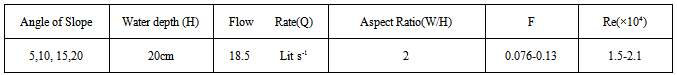
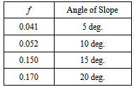
Experiments were carried outin a flume 8-m long, 0.4-m wide and 0.6-m deep with glass sidewalls. The flow depth was controlled during the experiments by a tailgate located at the end of the flume. The pools were located 5 to 6.7 m away from the channel entrance where the thickness of boundary layer was fully developed in the flume. The pools were madewithgravel with a median diameter (D₅₀) of 10 mm and angles of 5, 10, 15 and 20 degrees for the entry and the exit slopes based on data collected in alluvial channels in Iran. The wavelength of the two-dimensional bedform was 1.5 m for each run and the measurements were made at 14 sections along the flume, starting 10 cm upstream of the pool entry to 10 cm downstream of the pool exit. Figure 1 shows a schematic of laboratory setup.

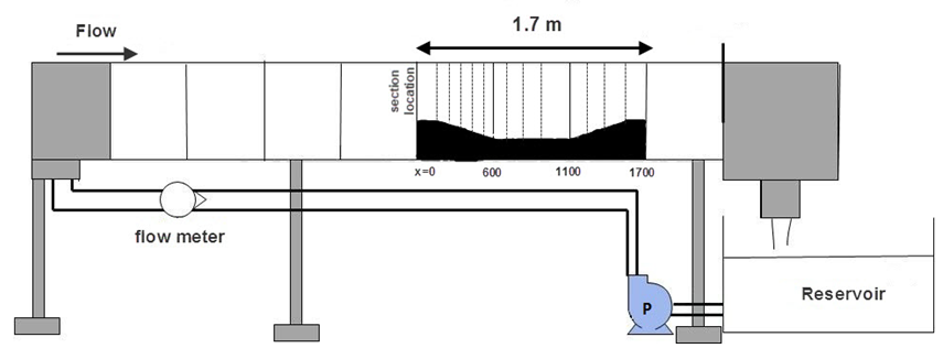Figure 1. labratuary setup

An ADV with a sampling rate of 200 Hz and sampling duration of 120 seconds was used to measure the velocity profiles. To obtain high quality data from the time series, ADV velocity data were filtered by the Goring and Nikora (12) algorithm. The summary of flow characteristics for each run is presented in Table 1.

A flowchart for the description of methodology is presented in Fig. 2.

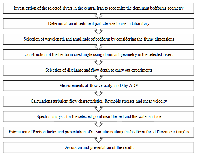Figure 2. flowchart of methodology description

Table 1. Flow characteristics of the experiment

The instantaneous velocity is presented as:

(1)

Where angle brackets shows double averaging operator, the tilde sign shows spatial variable and prime sign displays velocity fluctuations. Nikora et al.[17] defined the double averaged velocity as:

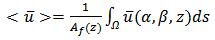(2)

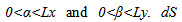Ω is the domain occupied by the fluid within a fixed region with the area of L_x × L_y at level z (assumed parallel to the bed). Function A_f(z) is defined as the void distribution between the lowest troughs and the highest crests of the roughness elements. Dummy variables α and β are such that is thehorizontal surface of integration[8]. For gravel-bed rivers, the dimensions of the spatial averaging domain should be much larger than gravel size and much smaller than bedform size. In this study and for an artificial pool of 1.5 m long, the selected length is 100 mm which is larger than the mean particle size (10 mm) and smaller than the length of the pool (1.5 m).

Since the ADV provides measurements at a specific point in space, the spatially-averaged value of the velocity can be determined as follows:

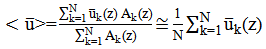(3)

Where N represents the number of subdomains and A_k(z) is the area of subdomain at elevation z. The momentum equation for 3D steady turbulent open-channel flows can be presented as:

(4)

Where u_i is theith component of the velocity; x_i, the ith direction; g, the gravitational acceleration; ρ, the density; p, the pressure; and ν, the kinematic viscosity. Application of the double-averaging operator <> to the time varying quantities and to the partial derivatives renders the Double-Averaged momentum equation (5):

(5)

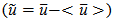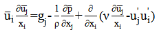
In above equations the over bar and angle brackets denote the time and spatial average of flow variables, respectively; the tilde denotes the perturbation in the flow variables caused by the elements of bed roughness, i.e., the difference between time-averaged () and double averaged () values; where is similar to the Reynolds decomposition . is the ratio between the area occupied by the fluid (A_f) and total area at elevation z. In this study, the value of is equal to 1. Equation (5) describes the relationship between the double-averaged flow properties and it accordinglycontains some additional terms in comparison tothe conventional time-averaged Navier-Stokes equations. These terms are form-induced stresses (), viscous (skin) friction (f_v), and form drag (f_D). The form-induced stresses appear as a result of spatial averaging just like turbulent stresses appear in the Reynolds-averaged Navier-Stokes equations as a result of time averaging. The form drag and viscous friction appear only in equations for the flow region below roughness crests. Since ADV cannot measure the flow velocity below gravel crest, f_v and f_D are not considered in this study. Theviscous drag (f_v) on the bed in equation (5) can be neglected for high roughness Reynolds numbers as well. Nikora et al., 2001; Nikora and McLean, 2001 showed that in hydraulically rough bed and large relative submergence, the viscous effects are negligible.

There are many physical phenomena producing data which are not deterministic. These random data must be described in terms of probability statements and statistical averages. Turbulent flow is an ergodic random process and power spectral density functions describe the general frequency composition of this process in terms of spectral density of its mean square value. To perform spectral analysis, several points from different velocity profiles were selected. These points located near the bed (z=6 mm) and near the water surface (z=160 mm) for four slope angles of the pools. Figure 3 shows the power spectra graphs in some selected points near the bed and the water surface. Kolmogoroff presented a model of approximately isotropic turbulence in which a -5/3 power law exists between frequency and turbulence spectrum in theso-called ‘inertial subrange’ for valid time series data. Figure 3 confirms the slope of -5/3 for all selected points.

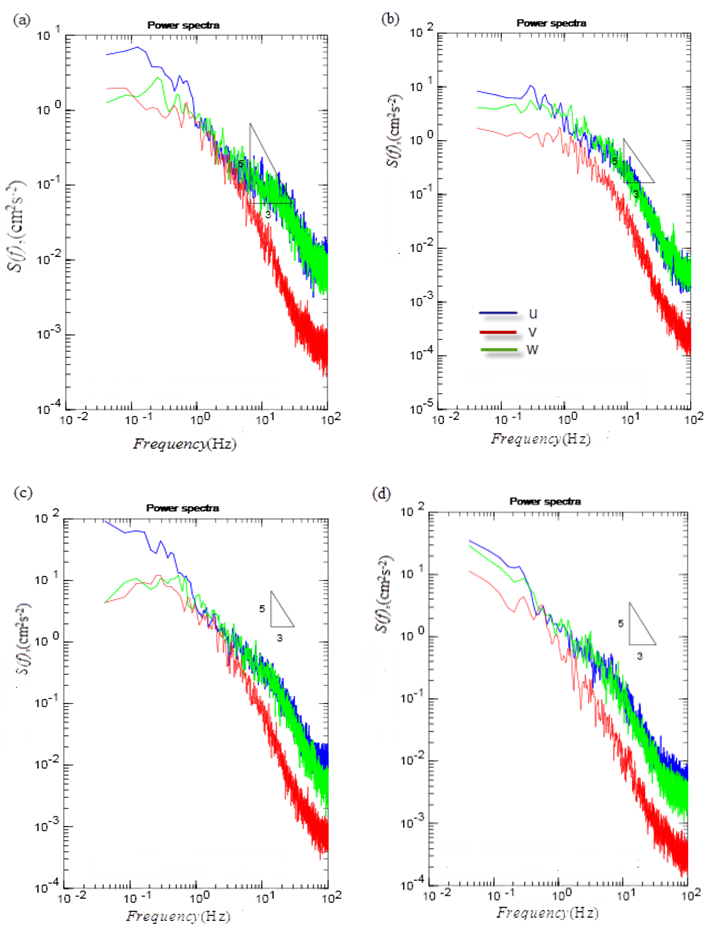Figure 3. Turbulence Spectrum of some points

3. Results

3.1. Shear Stress Distribution

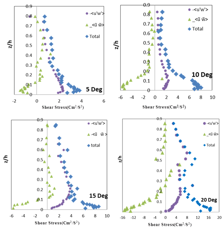
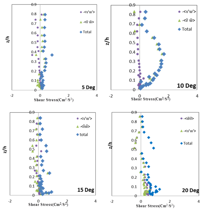
Reynolds shear stress, form-induced and total shear stress distributions derived from Double-averaged Navier-Stokes equations are presented in Figs. 4-6 for the streamwise, spanwise and vertical directions. The absolute values of the Reynolds and form-induced shear stresses were added to get total shear stress value. The viscous stress is neglected, therefore, it is not considered in the estimation of the total stresses. Despite of the fact that Reynolds stress has a concave shape in accelerating flow and a convex shape in decelerating flow (3, 13, 15), Fig. 4 shows a convex distribution for double-averaged Reynolds stresses for all four slope angles. This observation shows that the effect of decelerating flow is more important than accelerating flow over the pools due to the dominant effect of adverse pressure gradient along this bedform. Figure 4 also shows that the maximum Reynolds stress value increases when the slope angle of the pool increases due to increasing turbulence intensity. According to Fig. 4, form-induced stresses in the inner layer are of the same order of magnitude as the Reynolds stresses. Form-induced stresses largely contribute to total stresses, especially near the bed, confirming that the pool geometry influences the shear stress distribution. The negative sign of form-induced stress shows that the momentum flux is directed toward the bed.

The maximum total stress value for the 5- and 10-degree slopes is located at z/h=0.04 and z/h=0.27, respectively, where the maximum form-induced stress value occurs, however, the peak of the total stress for the 15- and 20-degree slopes occurs somewhere slightly above the maximum form-induced stress, which is in agreement with the results obtained by Franca et al.[9].

Nikora et al.[17] and Nikora and McLean[18] demonstrated that form-induced momentum fluxes are negligible in the outer layer and the double-averaged equations are identical to the time-averaged equations in this region. For the 5- and 10-degreeslopes at z/h>0.35 and z/h>0.48, respectively, the form-induced stresses are negligible and Reynolds stress values are dominant. For 15- and 20degree slopes, the form-induced stresses are around zero at z/h>0.6 and z/h> 0.57, respectively, and total stress values are completely influenced by Reynolds stress. These observations corroborate the results of Nikora et al.[17] and Franka et al.[9], finding negligible form-induced stress values near the water surface. Figure 4 also shows an extreme value of form-induced stress near the bed for the 20-degree slope where the flow separation occurs. Flow separation, which grows as the slope angle increases, plays a significant role on form-induced shear stress.

Figure 4. Shear Stress Distributions (XZ)

Mclean and Nikora[14] suggested that contributions of the form-induced stresses to the total momentumbudget in gravel bed flows with small relative submergence may be fairly low, even close to the roughness elements. On the other hand, Gimenez-Curto and Corniero Lera[10, 11] found that with decreasing the relative submergence, the form-induced stress might have more contribution to total stress than that of the Reynolds stress. Although the relative submergence (H/d₅₀) at the upstream of the pools is equal to 20, the total stress distributions are influenced by the form-induced stress, especially near the bed region in the XZ plane (Fig.4).

Figures 5 and 6 present shear stress distributions in the X-Yand Y-Zdirections, showing the peak values of Reynolds stress occur above the bed in four slope angles; however, the peak value increases when the pool slope angle increases. The slope angle affects the total shear stress distribution in the XY and YZ plane bydisplaying different patterns. Figure 5 reveals that the form-induced stress becomes the most dominant component of the total stress, when the slope angle increases. Also, the Reynolds stress plays a significant role in the XY plane, especially near the bed. However, the Reynolds shear stress contribution is similar to the form-induced stress ofthe total shear stress in the YZ plane. Considerable scatter in the total double-averaged stresses for the 20-degree slope couldbe due to the significant flow separation near the bed, showing negative values of form-induced stress resulting in an irregular distribution of total stress.

Figure 5. Shear Stress Distributions (XY)

Figure 6. Shear Stress Distributions (ZY)

3.2. Friction Factor

Nikora et al.[17] derived the following relationship for the hydraulic friction factor (f) using the double-averaging method:

(6)

This relation was used to estimate the friction factor f over the pool where the shear velocity (u_*) was determined using theboundary layer characteristics method (1). The results presented in Table 2 show that the friction factor value increases when the slope angle increases, confirming the results of Figure 4 where the total stress increases as the pool slope increases.

Figure 7 shows the estimated friction factors over the pool at the central axis and ata distance of 5 cm away from the sidewall of the flume. Accordingly, an increase in the slope angle from 5 to 10 degrees causes a slight change in the friction factor, however, by increasing the slope angle from 10 to 15 or from 15 to 20 degrees modifies the friction factor considerably. Fig. 7 reveals that the effect of accelerating and decelerating flows on the friction factor is not significant forsmall slope angle (e.g., slope of 5 degrees). The maximum friction factor occurs at the end of the entry slope of the pool where the turbulence is high and the influence of separation flow is significant.

Table 2. Spatially averaged Friction Factor (f)

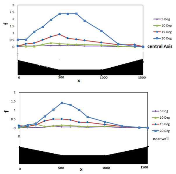Figure 7. Friction Factor f in central axis and near flume wall

4. Conclusions

In this study, pools were constructed usinggravel with a median diameter (D₅₀) of 10 mm, slope angles of 5,10,15 and 20 degrees at pool entry and exit and awavelength of 1.5 (as observed in several investigations in alluvial channels in Iran) to understand the influence of pool geometry on the distribution of shear stress and the estimation offriction factor. Double-averaged Navier–Stokes equations were applied to present the distributions of form induced stress and Reynolds stress as well as the estimation of friction factor. Results revealed that pool geometry influences differently the total shear stress distributions in the three directions. In the streamwise direction, the pool geometryeffect is notablenear the bed where the form-induced shear stress and the Reynolds stress play significant roles on the total shear stress. In the vertical and spanwise directions, the form-induced shear stress reveals a more significant contribution than the Reynolds stress on the total shear stress. The friction factor is influenced significantly by larger slope angles due to larger separation zones downstream the pool entry.

The results of this paper were compared with some studies over gravel bedforms with different geometries and crest angles. Motamedi et al (2012) observed no flow separation over low-angle dunes, however, they observed it for the crest angle 38 degrees. Nasiri et al (2013) confirmed the observation of flow separation for the high crest slope of 28 degrees over sharp-crest dune. The flow separation was clearly observed for the crest angles of 15 and 20 degrees over the pools in this study.

Reynolds stresses were affected by separation zone, increasing by the crest angle of the pools, confirming Nasiri et al (2013) results. Total double-averaged stresses for the crest slope of 20-degree displayed higher values in comparison with low crest angles with some data scatter due to significant flow separation near the bed. Nelson et al (1993) and Nasiri et al (2013) observed zero and slightly negative Reynolds stress values near the water surface stating that bedform geometry plays no role on the layer near the free surface. This finding was confirmed over the pools with different crest angles in this study.

The pool roughness features also create high flow resistance values compared tolower-gradient channels, as illustrated by the Darcy-Weisbach friction factors measured here. The spatial variation in friction factors in the study, with the lowest values insmall crest slope and the highest along large one (20 degree), supports Wohl and Thompson’s (2000) model of energy dissipation in step-pool channels[21]. Wohl and Thompson (2000) suggest that the wake-generated turbulence and form drag of step-pool reaches leads to higher energy dissipation relative to more uniform-gradient reaches such as low-crest slope that are dominated by bed-generated turbulence and skin friction.

Notation

D₅₀ = tunnel diameter (m)

F = Froude number (-)

f = friction factor(-)

g = gravity acceleration (ms^-²)

u= velocity (ms^-1)

u_*= shear velocity (m s^-1)

P = pressure (pa)

R = Reynolds number (-)

W/H = aspect ratio (-)

H/D₅₀= relative submergence(-)

ρ = density (kg m^-3)

ν = fluid kinematic viscosity(m²s^-1)