Kristen Pineda, Lubo Liu
Department of Civil and Geomatics Engineering, Lyles College of Engineering, California State University Fresno, Fresno, CA 93740
Correspondence to: Lubo Liu, Department of Civil and Geomatics Engineering, Lyles College of Engineering, California State University Fresno, Fresno, CA 93740.
| Email: |  |
Copyright © 2012 Scientific & Academic Publishing. All Rights Reserved.
Abstract
To investigate arsenic distribution, a prevailing problem in drinking water, arsenic concentrations in the drinking water supply for the southern San Joaquin Valley were mapped to show both current and historical concentration trends. This research was also to analyze the significance of the effect of water quality and environmental factors on arsenic concentrations in groundwater. These well construction factors included the total well depth, total length of the annular seal, average screened interval depth, as well as both iron and manganese concentrations in selected wells. The results of the correlation testing between arsenic and iron and manganese concentrations provided for a very weak correlation. Correlations between the arsenic concentration and well construction were much stronger. Different statistical methods were used to test the correlations between the arsenic concentration and the three well construction parameters. Pearson’s r provided the weakest correlations with the correlation coefficients of 0.2237, 0.122, and 0.228, respectively. Kendall’s tau and Spearman’s results show stronger correlations with coefficients of 0.302, 0.13, and 0.311. Using Spearman’s rho, the correlation coefficients were 0.405, 0.155, and 0.414. Kendall’s tau was not determined to be statistically significant at a 5% confidence interval for all three variables. Spearman’s rho was determined to be statistically significant at a 5% confidence interval for well depth and average screened depth.
Keywords:
Arsenic, Groundwater, Well Construction Parameters, Correlation
Cite this paper: Kristen Pineda, Lubo Liu, Arsenic in Drinking Water Supply Wells: A Geographical and Statistical Investigation of the Southern San Joaquin Valley, International Journal of Hydraulic Engineering, Vol. 2 No. 6, 2013, pp. 121-132. doi: 10.5923/j.ijhe.20130206.01.
1. Introduction
Arsenic is a prevailing problem in drinking water, especially in California’s San Joaquin Valley. Human exposure to arsenic is predominantly through “ingestion or inhalation”[1] and arsenic exposure is primarily cumulative [2]. Inorganic arsenic generally has a higher toxicity than organic arsenic and toxicity also depends on the binding form of the metalloid[3]. Regulations focused on arsenic exposure through the ingestion of drinking water place emphasis on long-term and chronic exposure. Exposure to inorganic arsenic, which is more prevalent in drinking water, can also be acute. Inorganic arsenic consumption is known to have carcinogenic effects on the following: bladder, kidneys, liver, lungs, nasal passages, prostate gland, and the skin[3, 4, 5]. Inorganic arsenic also has non-carcinogenic health effects on the following bodily systems: cardiovascular, endocrine, immunological, neurological, and pulmonary[4]. In drinking water, arsenic is more concentrated in groundwater supplies as opposed to surface water sources. Public water systems with arsenic-contaminated sources are much more prevalent in the western part of the United States[6]. Despite geographic trends, there still may be arsenic “hotspots” throughout the country[6]. Stricter regulations were recently adopted that lowered the Maximum Contaminant Level (MCL) for arsenic in drinking water. This reduction in allowable levels of arsenic has made many public water systems in the San Joaquin Valley out of compliance with both state and federal regulations. California’s revised arsenic Maximum Contaminant Level, which was identical to the federal Maximum Contaminant Level of 0.010 mg/L or 10 ppb, went into effect on November 28, 2008[7]. In a survey of water quality data, the California Department of Public Health-Drinking Water Program found that California had approximately 600 drinking water supply sources with arsenic levels above Maximum Contaminant Level[7]. Many of these water systems are required to either acquire new sources of drinking water supply or provide treatment for their existing sources. Approximately 40 percent of California’s residents use groundwater as their drinking water source and “contaminated groundwater results in treatment costs, well closures, and new well construction which increases costs for consumers”[8].This paper focuses on arsenate and arsenite since they are the most prevalent forms of inorganic arsenic in groundwater [3, 9, 5]. Arsenic movement in soil can be affected by several factors including the soil pH, the redox potential, and the adsorbing components within the soil[3, 10]. However, mobility is also affected by the competing anions of aluminum, calcium, iron, manganese, and magnesium[3]. These anions affect adsorption site availability[3]. Iron (III), aluminum (III) and manganese (III/IV) all form both oxides and hydroxides that adsorb to various arsenic compounds[3]. However, these arsenic compounds typically bind to iron and manganese under reducing conditions[3]. Fate and transport of arsenic in groundwater is impacted by many processes including groundwater hydrodynamic conditions, arsenic sources, sorption/desorption, soil properties, and the abundance of co-contaminants such as irons and manganese[11]. Immobilization of arsenic in groundwater occurs through sorption of arsenic onto the sediment deposits of the aquifer. This is a partitioning process which is influenced by redox conditions since the oxidation state dictates the adsorption extent. Arsenic mobilization occurs in reduction zone for iron and manganese and is “sequestered in the oxidations zones”[11]. However, sequestration also occurs in the reducing zone for sulfides. This sequestration is reliant on the speciation of arsenic in the groundwater[11]. Elevated arsenic levels are found in both oxidizing and reducing conditions in groundwater aquifers[12].The objective of this research was to map arsenic concentrations in the drinking water supply for the southern San Joaquin Valley to show both current and historical concentration trends. The secondary objective was to analyze the significance of the effect of water quality and environmental factors on arsenic concentrations in groundwater. These well construction factors included the total well depth, total length of the annular seal, average screened interval depth, as well as both iron and manganese concentrations in selected wells. Wells were selected from the twenty-five water systems, which were chosen as representative systems from throughout the Tulare Lake Hydrologic Region within the confines of the San Joaquin Valley Groundwater Basin. Specific wells were selected based on the availability of well construction data as well as the availability and abundance of water quality data in regards to arsenic, iron, and manganese concentrations. These wells were deemed to be representative of their respective system and of the region. Furthermore, different factors including well construction parameters and the iron and manganese concentrations, were analyzed to determine their respective statistical significance on the arsenic concentration in the drinking water supply.
2. Description of Study Area
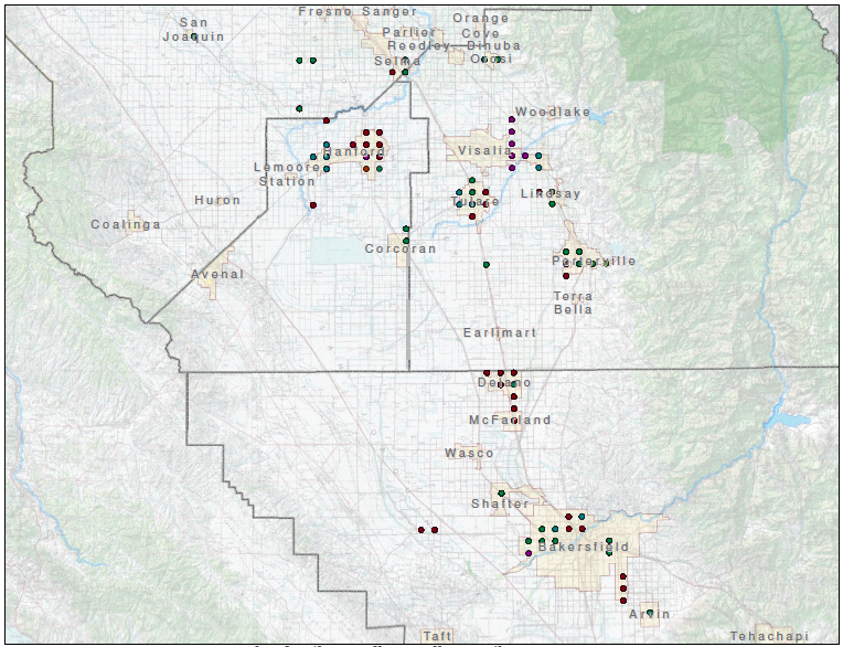 | Figure 1. Well Cluster Locations |
The southern portion of the San Joaquin groundwater basin excluding the Pleasant Valley sub-basin is the focus of this research. According to the Department of Water Resources, the San Joaquin Valley accounts for 48% of all groundwater use in the state[13]. This use is predominately agricultural with some municipal uses[13]. Water quality and well construction data was gathered for select drinking water supply wells from 25 public water systems in the southern San Joaquin Valley (Figure 1). These public water system were selected based on their varying geographic locations and water supply quality and should be representative of the majority of public water systems within the study area.Streams and percolation from irrigation are the predominate source of groundwater recharge in the sub-basins and groundwater quality is generally poor with high concentrations of total dissolved solids. Furthermore, localized areas have increased concentration of selenium and boron[13]. In the eastern region of the sub-basin, flood basin deposits cause poor drainage and percolation which results in a buildup of applied irrigation water in the shallower zones.
3. Methodology
The methods used in this research involve data collection and analysis with several statistical schemes.
3.1. Data Collection
The data collected included water quality information, both historic and current, on hundreds of public drinking water supply wells within the southern San Joaquin Groundwater Basin. This included public drinking water supply wells within both the San Joaquin River and Tulare Lake Hydrologic Regions as well as in the following groundwater sub-basins: Kaweah, Kings, Kern, Pleasant Valley, Tulare Lake, Tule, and Westside. Geographically speaking, this encompassed an approximate area from the City of Fresno to the southern boundary of the Central Valley and the valley floor bounded on the east and west by the Sierra Nevada mountain range and the Coast Range foothills, respectively.The Groundwater Ambient Monitoring and Assessment program (GAMA) maintained by the State Water Resources Control Board (SWRCB) called for sampling of untreated groundwater from a variety of different wells to include environmental monitoring wells as well as drinking water supply wells[8]. A publically available database compiling these water quality sampling results with water quality data from different regulatory agencies and other entities was created as part of the program. The current data contributors include the following: California Department of Pesticide Regulation, California Department of Public Health, California Department of Water Resources, Lawrence Livermore National Laboratory, Regional Water Quality Boards, State Water Resources Board, and the United States Geological Survey[8]. This database was developed, in part, to “to increase the availability of groundwater quality information to the public”[8]. As one of four components in the GAMA program, GeoTracker GAMA data base with over 100 million analytical results, well logs and water levels from over 200,000 wells, was used in this research. All well logs available in the database are strict for environmental monitoring wells and do not include any exact locational or well construction data for drinking water supply wells. Only approximate well locations were provided for drinking water supply wells. Figure 1 shows the locations of the well clusters as found in GeoTracker Gama.Water quality samples for iron and manganese were paired to arsenic samples collected on the same date and from the same well. Both iron and manganese are secondary standards which are less stringently regulated and have different monitoring requirements than arsenic.
3.2. Statistical Analysis
Statistical analysis for this project was completed using the Scout 2008 version 1.0 and the SPSS Statistics software packages. Censored data is dealt with through omission or substitution. A positive bias in data trends is likely to occur when censored data is omitted from the data set. However, deletion of these values can potentially highlight variances in the upper quantiles of a data set which may not have been seen if the censored values were present[14]. For this round of testing, censored data was replaced with estimated numerical values generated using regression-on-order statistics which assumed a lognormal distribution of data. These numerical replacements were generated using the Scout 8 software. The potential distributions of all the water quality data were evaluated. The Shapiro-Wilk and Lilliefors tests were used to test for normal distribution. Smaller data subsets were created by grouping groundwater basins. The Shapiro-Wilk and Lilliefors tests were also utilized to test for lognormal distribution using estimated lognormal ROS values. Smaller data subcategories were created and grouped by groundwater basins. The Anderson-Darling and Kolmogorov-Smirnov tests were used to evaluate gamma distributions amongst the arsenic, iron, and manganese datasets.
3.3. Data Correlation
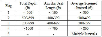
In this research, all available arsenic data that had either a paired iron or manganese sample collected on the same day from the same well was used to investigate if there was a correlation between the concentrations of constituents within drinking water supplies. Water quality data was included even if no well construction information was available. Correlation between arsenic/iron concentrations and arsenic/manganese concentrations were calculated using graphic and nonparametric methods. In order to measure the correlation between the arsenic concentration and one of the well construction factors, the other two well construction factors needed to be controlled. The total well depth was divided into four subgroups based on depth and given a flag, as was the annular seal depth. The average of the screened interval depth was calculated and the data was placed in subgroups and flagged as well. For wells with multiple screened intervals which encompassed many ground water zones, a separate subgroup was created. In the end there were five subgroups for the screened interval factor. Table 1 below breaks down the different flagging criteria.Table 1. Well Construction Flagging
 |
| |
|
Multiple correlation testing was conducted for the well construction factors, controlling for different flags within the different factors each time
3.4. Concentrations Mapping
Mapping of historic and current arsenic concentrations was accomplished through a geographic information system (GIS). Topographical and other maps were compiled for the project area. These maps were reviewed for accuracy and emphasis was placed on verifying groundwater sub-basin boundaries. The overlay maps were prepared for use in documenting historical and current water quality concentration trends. These maps were then imported into ArcGIS to create concentration distribution maps for arsenic, iron, and manganese. The iron and manganese maps were created to compare their concentration distributions with arsenic to further investigate their correlations with arsenic.
4. Results and Discussion
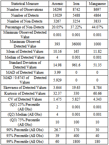
The dataset included 16,296 arsenic samples of which 3,267 of them, or approximately 20%, were censored data values. There were 8,742 iron samples that could be paired to a corresponding arsenic sample. Of these, 3,254, or approximately 37%, were censored data values. There were 8,697 manganese samples that could be paired to a corresponding arsenic sample of which 4,864, or approximately 44%, were censored data values. Statistical calculations for each constituent are displayed below in Table 2.Censored values were estimated using regression-on-order statistics assuming a normal, lognormal, or gamma distribution. The Scout 2008 software package allows for estimated using a uniform random variable. Estimated values using gamma regression-on-order statistics ranged from to approximately 1.269 for arsenic, 176 for iron, and 6.9 for manganese. These values were estimated assuming a gamma distribution without the censored value and appear to be a better fit that the normal and lognormal regression-on-order statistics. These estimations can be erroneous if a gamma distribution cannot be verified. Estimated values using uniform random variables were typically in the range of 10-3. The values are generated using a uniform random variable generator as part of the Scout 2008 software. These values appeared to be a better fit than both the normal and lognormal regression-on-order statistical estimates. Table 2. Statistical Measures
 |
| |
|
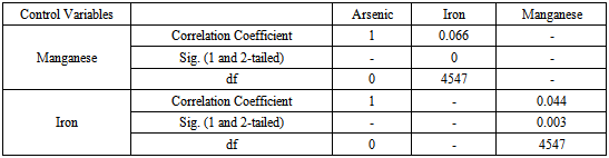
Outlier tests were performed on each sub-basin data set. Censored data was omitted in the first tests and, for the second tests, a value equal to one half the detection limit was substituted in. Both rounds of tests identified the same potential outliers. Outliers were left in for further statistical analysis. The Rosner’s Test was used for all analysis since the Dixon’s Test can only be used for datasets of less than 25. When divided by sub-basin, the dataset still exceeded the maximum size and, when divided by well name, there were not enough samples for analysis. The results of the correlation testing between arsenic and iron and manganese concentrations provided for a very weak correlation between arsenic and iron and between arsenic and manganese. Table 3 below summarizes the results of the correlation testing between water quality variables. As expected, the parametric equation provided the weakest, almost zero, correlation at 0.081 and 0.064 for iron and manganese, respectively. Kendall’s tau and Spearman’s rho provided stronger correlations. Using Kendall’s tau, the correlation coefficients were 0.134 and 0.152 for iron and manganese. Using Spearman’s rho, the correlation coefficients were 0.158 and 0.177 for iron and manganese. Each coefficient calculated in the three tests was scaled differently. Kendall’s tau was not determined to be statistically significant at a 5% confidence interval. Spearman’s rho was not determined to be statistically significant at a 5% confidence interval.The lack of a correlation between arsenic and iron/manganese is visually apparent in Figures 2and 3 below and is also shown in the relatively flat trend line.Testing involving partial correlations included controlling for other variables. In these tests, the controlling variable was the other water quality constituent. Partial correlation provided a weak correlation coefficient at 0.066 for iron and 0.044 for manganese. Table 4 summarizes the results of the partial correlation testing. Correlations were based on the entire dataset which included sample from wells with a wide variety of different construction features. Had well construction data been available for all wells in the study location, it would have been possible to run correlations between similarly constructed wells, thus controlling for other variable that may be influencing arsenic levels. Furthermore, the availability of well boring logs would have allowed for further accuracy as the borehole-specific geology and the supplying aquifers could have been controlled.Table 3. Water Quality Correlations
 |
| |
|
Table 4. Water Quality Partial Correlations
 |
| |
|
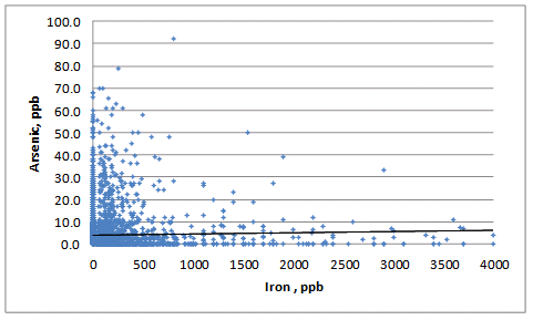 | Figure 2. As vs. Fe graph |
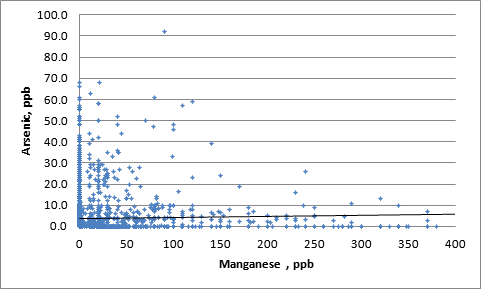 | Figure 3. As vs. Mn graph |
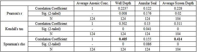
Correlation testing between average arsenic concentrations and well construction factors involved the use of the same methods described above, including Pearson’s r. Correlations between arsenic concentration and well construction were much stronger than the correlation between arsenic concentrations and iron and manganese. Like the previous testing, Pearson’s r provided the weakest correlations at 0.2237, 0.122, and 0.228 for well depth, annular seal length, and average screened depth, respectively. Kendall’s tau and Spearman’s rho provided stronger correlations. Using Kendall’s tau, the correlation coefficients were 0.302, 0.13, and 0.311 for well depth, annular seal length, and average screened depth. Using Spearman’s rho, the correlation coefficients were 0.405, 0.155, and 0.414 for well depth, annular seal length, and average screened depth. Kendall’s tau was not determined to be statistically significant at a 5% confidence interval for all three variables. Spearman’s rho was determined to be statistically significant at a 5% confidence interval for well depth and average screened depth. This value was not significant for annular seal length. Table 5 summarizes the results of the correlation testing between well construction variables.Table 5. Well Construction Correlations
 |
| |
|
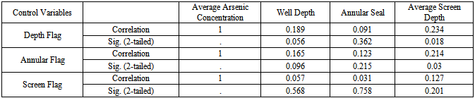
Figures 4, 5, and 6 are provided to visually asses the strength of the correlations between different well construction factors and the arsenic concentration.Testing involving partial correlations included controlling for other well construction variables including: depth, annular seal length, and average screen depth. Partial correlation provided much weaker correlation coefficients than the previous correlation tests. Table 6 summarizes the results of the partial correlation testing. Table 6. Well Construction Partial Correlations
 |
| |
|
 | Figure 4. As vs. well depth |
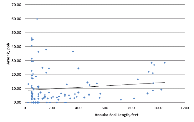 | Figure 5. As vs. annular seal |
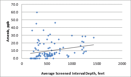 | Figure 6. As vs. screened interval |
Arsenic concentration data was available starting in 1978; however, there were less than 20 sample results during the five year period from 1978 to 1983. The number of available sample results increased significantly after that period with over 160 samples in the 1984 calendar year alone. Due to this availability, concentration distribution maps were created each year from 1984 to 2011. A discussion of these concentration distribution maps is provided below.In 1984, the map show relatively constant arsenic concentrations of 10 to 20 ppb throughout the project area. There was a lower concentration area in the northeast corner of up to 10 ppb and clusters of higher concentrations (20 to 30 ppb) around the City of Hanford and the City of Tulare. In actuality, only three of the 160 samples had detectable levels of arsenic (ranging from 11 to 28 ppb) and the rest of the data was censored data with multiple laboratory detection limits, ranging from <1 to <30 ppb. This high percentage of censored data skewed the concentration around the three detected samples and around the samples with the highest laboratory detection limit. Due to these factors, this map is deemed inaccurate and not representative of the project area.In 2010, there were 936 samples collected, of which 737 had detectable concentration. The detectable concentration ranged from 0.7 to 89 ppb. Higher concentration contours were found around the expected cities based on previous years. However, these contours went further east than expected since the lower concentration wells from Portville that usually act as a boundary condition were not sampled. Lower concentrations were found as expected around Lemoore and, erroneously around Corcoran which was not sampled. In 2011, 669 of 1,099 samples had detectable levels of arsenic. Concentrations ranged from 0.8 to 130 ppb. Contouring appeared as expected. In the north, higher concentrations were found in Hanford, Riverdale, and Caruthers, with lower concentrations found in Lemoore and along the east side. In the south, higher concentrations were present near Delano and Arvin, with the lower concentrations around Bakersfield. Average arsenic concentrations are mapped for selected water systems that appeared to have an influence on concentration contour shifts or those which appeared to act as a boundary condition. These average concentrations were graphed with respect to plus/ minus one standard deviation as well as all the individual well data.Figure 7 shows the average arsenic concentration for Arvin community services district with respect to +/- one standard deviation. Average arsenic concentrations remained relatively consistent over time. This well was constructed to a total depth of 730 feet with an annular seal to a depth of 50 feet. The screened interval of this well runs from 350 to 700 feet, with an average depth of 525 feet. This well had over 70 arsenic samples collected between February 1988 (40 ppb) and September 2011 (30 ppb). The average arsenic concentration was approximately 29.5 ppb. Arsenic concentrations fluctuated throughout each calendar year and have exhibited a slight general decrease. Buttonwillow Community Services District provides a domestic water supply to the City of Buttonwillow. Well construction information was available for all of the wells with available water quality data. The well 1510011-001 was constructed to a total depth of 500 feet with an annular seal to a depth of 300 feet. The start of the screened interval of this well was unavailable and assumed to start at the base of the annular seal. The depth of the screen in 400 feet, with an average assumed depth of 350 feet. The approximate depth to the Corcoran Clay layer is roughly 350 to 400 feet. This well had approximately 10 arsenic samples collected between July 1990 (11 ppb) and June 2009 (3.4 ppb). The average arsenic concentration was approximately 5.7 ppb. Arsenic concentrations fluctuated throughout each calendar year and have exhibited a general decrease. The well 1510011-003 was constructed to a total depth of 540 feet with an annular seal to a depth of 65 feet. The start of the screened interval of this well was unavailable and assumed to start at the base of the annular seal. The depth of the screen in 410 feet, with an average assumed depth of 238 feet. The approximate depth to the Corcoran Clay layer is roughly 350 to 400 feet. Arsenic samples for this well were collected between December 1991 (12.1 ppb) and June 2009 (6.8 ppb). The average arsenic concentration was approximately 9.3 ppb. Arsenic concentrations fluctuated throughout each calendar year and have exhibited a general decrease. 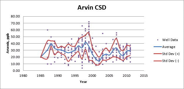 | Figure 7. Arvin CSD - average As concentrations |
Figure 8 shows the average arsenic concentration for the city of Corcoran with respect to +/- one standard deviation. Average arsenic concentrations generally decreased over time.Figure 9 shows the average arsenic concentration for Hanford city with respect to +/- one standard deviation. Average arsenic concentrations slightly decreased over time. The City of Lemoore water system provides a domestic water supply to the City of Lemoore. Well construction information was available for seven of the wells with available water quality data. Figure 10 shows the average arsenic concentration for this water system with respect to +/- one standard deviation. Average arsenic concentrations remained relatively consistent over time. 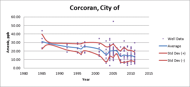 | Figure 8. City of Corcoran - average As concentrations |
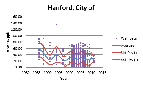 | Figure 9. City of Hanford - average As concentrations |
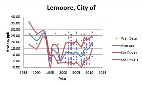 | Figure 10. City of Lemoore - average As concentrations |
Figure 11 shows the average arsenic concentration for Lindsay city water system with respect to +/- one standard deviation. Average arsenic concentrations remained relatively consistent over time. The City of Porterville water system provides a domestic water supply to the City of Porterville. Well construction information was available for 19 of the wells with available water quality data. Figure 12 shows the average arsenic concentration for this water system with respect to +/- one standard deviation. The City of San Joaquin water system provides a domestic water supply to the City of San Joaquin. Well construction information was available for one of the wells with available water quality data. Figure 13 shows the average arsenic concentration for this water system with respect to +/- one standard deviation. Average arsenic concentrations remained relatively consistent over time. Well construction information was obtained for well 1010034-003. This well was constructed to a total depth of 589 feet with an annular seal to a depth of 56 feet. The screened interval of this well runs from 210 to 510 feet, with an average depth of 360 feet. The approximate depth to the Corcoran Clay layer is roughly 450 to 500 feet Arsenic samples for this well were collected between September 1985 and October 2010. Arsenic concentrations ranged from non-detectable to less than 10 ppb. The Average arsenic concentration was 6.28 ppb.The City of Tulare water system provides a domestic water supply to the City of Tulare. Well construction information was available for 13 of the wells with available water quality data. Figure 14 shows the average arsenic concentration for The City of Tulare water system with respect to +/- one standard deviation. 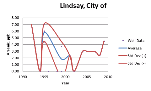 | Figure 11. City of Lindsay - average As concentrations |
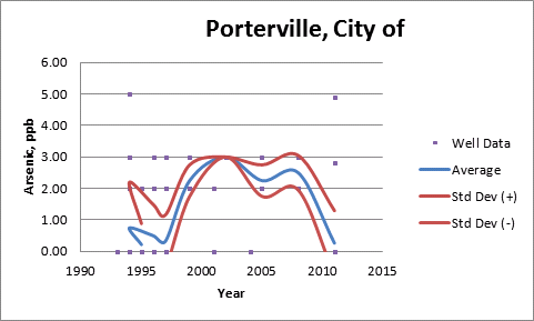 | Figure 12. City of Porterville - average As concentrations |
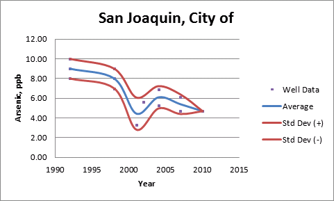 | Figure 13. City of San Joaquin - average As concentrations |
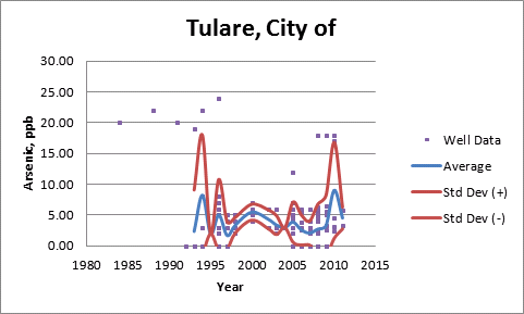 | Figure 14. City of Tulare - average As concentrations |
The monitoring wells were constructed to a total depth of about 600 feet with an annular seal to a depth of 300 feet. The screened interval of this well runs from 320 to 600 feet, with an average depth of 460 feet. The approximate depth to the Corcoran Clay layer is roughly 200 to 300 feet. Arsenic samples for this well were collected between May 1991 (<10 ppb) and December 2010 (non-detectable). The average arsenic concentration was approximately 6.5 ppb. Arsenic concentrations fluctuated but have remained relatively constant.
5. Conclusions
The arsenic concentration distribution was inconsistent and not representative of the entire project area. Shifts of higher concentration contours repeatedly occurred along the west side of the project area due to the fact that many communities in western Fresno County and Kings County utilize surface water as their primary source of drinking water supply. The lack of drinking water supply wells along the western side meant that the higher concentrations with the central part of the project area significantly influenced the west side since no other concentration boundary existed. High arsenic concentrations in the wells serving the cities of Riverdale and Hanford primarily controlled the west side. This was plainly evident in that the alternating high and low concentration contours of the west side coincided with whether these wells, or a combination thereof, were sampled in a given year. Wells serving the cities of Lemoore and Bakersfield, along with the communities along the eastern boundary of the project area were the dominate factors in the shape of the low concentration contours. Again, this was evident in that the contours shifted according to which cities wells had been samples in a given year. In addition, prior to about 1992, there were not an abundance of arsenic samples on file from multiple water systems and the high method detection limits of the laboratories, detectable sample results comprised of a few systems with highest concentrations of arsenic. The maps began to be more representative with the more sampling. New lower concentration arsenic wells provided a boundary in the west, while Porterville, Tulare, and other cities provided the boundary in the east. The research of correlations between arsenic concentrations and other environmental factors remains incomplete and inconclusive as well. Water quality correlations were based on the entire dataset which included samples from wells with a wide variety of different construction features. The widely varying construction and lack of information on the specific construction made it impossible to control for different features, aquifers, and geology. If these factors could have been better controlled, it is possible that correlations between arsenic and iron/manganese amongst similarly constructed wells could be seen. As it stands, there are too many uncontrolled variables in this research to definitively establish a correlation. Arsenic concentrations either remained relatively constant or generally decreased across each water system as a whole, and not specifically by each individual well. This overall generalized decrease is most likely a result of the water systems drilling new sources of drinking water supply and not anything to do with naturally occurring arsenic levels within the aquifer itself. These new sources are more likely to have greater depth, have greater consideration put into the intervals of the screened casing, and pull from deeper, better quality aquifers. Water systems along the eastern boundary of the project remained consistent over time while arsenic levels typically below the maximum contaminant level. The arsenic in the region is naturally occurring, specifically in relation to historic lakebeds, in which proximity to typically have higher levels of arsenic in the shallower aquifers. Seasonal fluctuations were apparent and are related to the rising and falling of the water table elevation.Further analysis into the statistical correlations of environmental factors is recommended if well boring logs or other information pertinent to well construction, the geology of the well boreholes, surrounding aquifer, and location of any confining layer or aquitards can be obtained.
References
| [1] | http://en.wikipedia.org/wiki/Arsenic |
| [2] | K. Gehle, “ATSDR Case Studies in Environmental Medicine,” U.S. Department of Health and Human Services Agency for Toxic Substances and Disease Registry, 2009. |
| [3] | M. Bissen, F. Frimmel, “Arsenic – a Review. Part 1: Occurrence, Toxicity, Speciation, Mobility,” Acta hydrochim hydrobiol, 31(1), pp. 9-18, 2003. |
| [4] | “Technical Fact Sheet: Final Rule for Arsenic in Drinking Water,” 2001. EPA-815-F-00-016.http://water.epa.gov/lawsregs/rulesregs/sdwa/arsenic/regulation_techfactsheet.cfm. |
| [5] | K. Kerri, Water Treatment Plant Operation 2 (5), University Enterprises, Inc, 2006. |
| [6] | “Fact Sheet: Drinking Water Standard for Arsenic,” 2001. EPA-815-F-00-015.http://water.epa.gov/lawsregs/rulesregs/sdwa/arsenic/regulations_factsheet.cfm. |
| [7] | USDA-ARS U.S. Salinity Laboratory, “Arsenic in Drinking Water: MCL Status,”http://www.cdph.ca.gov/certlic/drinkingwater/Pages/Arsenic.aspx |
| [8] | State Water Resources Control Board - Geotracker GAMA, http://www.waterboards.ca.gov/gama/geotracker_gama.shtml |
| [9] | Arsenic Treatment Technology Evaluation Handbook for Small Systems, EPA 816-R-03-014, 2003. |
| [10] | P. Masscheleyn, R. Delaune & W. Patrick, “Effect of Redox Potential and pH on Arsenic Speciation and Solubility in a Contaminated Soil, “Environmental Science & Technology, 25, pp. 1414-1419, 1991. |
| [11] | J. Reisinger & J. Hering, “Remediating Subsurface Arsenic Contamination with Monitored Natural Attenuation,” Environmental Science & Technology, pp. 458A-464A, 2005. |
| [12] | P.L. Smedley & D.G. Kinniburgh, “A review of the source, behaviour and distribution of arsenic in natural waters,” Applied Geochemistry, 17, pp. 517–568, 2002. |
| [13] | CA Department of Water Resources, “Bulletin 118: California’s Groundwater,” 2003. |
| [14] | D. Helsel, “Advantages of nonparametric procedures for analysis of water quality data,” Hydrological Sciences, 32(2), pp. 179-190, 1987. |
 Abstract
 Reference
 Full-Text PDF
 Full-text HTML