Tcheukam-Toko D.1, Mokem-Chetchueng M2, Mouangue R.1, Beda T.2, Murzyn F.3
1Department of Energetic Engineering, University Institute of Technology, P. O. Box 455 Ngaoundere, Cameroon
2Department of Physics, Faculty of Sciences; University of Ngaoundere, P. O. Box 454 Ngaoundere, Cameroon
3ESTACA, Campus Ouest, Parc Universitaire de Laval – Changé, Rue Georges Charpak, BP 53061 Laval Cedex 9, France
Correspondence to: Tcheukam-Toko D., Department of Energetic Engineering, University Institute of Technology, P. O. Box 455 Ngaoundere, Cameroon.
| Email: |  |
Copyright © 2012 Scientific & Academic Publishing. All Rights Reserved.
Abstract
Numerical analysis was performed for the two-dimensional open-channel flow over an obstacle generating a hydraulic jump. Special attention has been paid for the friction effect near the obstacle, and for the interaction between the vortex structures and the air bubbles. The influence of the second fluid (air); has permitted to consider the air-water emulsion as a compressible biphasic fluid characterized by a void fraction. The volume of fluid (VOF) model, coupled to the turbulent model has been applied a standard κ-ε two equations model and the two-dimensional Reynolds Averaged Navier–Stokes (RANS) equations are discredited with the second order upwind scheme. The SIMPLE algorithm, which is developed using control volumes, is adopted as the numerical procedure. Calculations were performed for a wide variation of the Reynolds numbers (Re) and the Froude numbers (Fr), corresponding to different flows. The results reveal that with increasing Reynolds number, the gas phases have more influence on the liquid phases. In the upstream zone from the obstacle, the boundary layer thickness decrease with the increasing Reynolds number while the height of the recirculation zone is increasing in the downstream from the obstacle. The void fraction profiles show two regions justifying a diffusion equation. Comparison of numerical results with the experimental data available in the literature is satisfactory.
Keywords:
Hydraulic jump, Open-channel flow, Void fraction, Biphasic flow, Pressure field, Dynamic field, Boundary layer, VOF, CFD
Cite this paper: Tcheukam-Toko D., Mokem-Chetchueng M, Mouangue R., Beda T., Murzyn F., Characterization of Hydraulic Jump over an Obstacle in an Open - Channel Flow, International Journal of Hydraulic Engineering, Vol. 2 No. 5, 2013, pp. 71-84. doi: 10.5923/j.ijhe.20130205.01.
1. Introduction
The hydraulic jump is a rapid and sudden transition from a high-velocity supercritical flow to a subcritical flow. It is characterized by the presence of large vortex, the projections of water-package to the free surface carrying air and the important dissipative energy. The comprehension and opinion of hydraulic jump reveal its importance in hydraulic. In fact, its properties are based on the impact structures or the restoration of rivers. It is used in the hydraulic construction like an energy dissipater, allowing to reduce as maximum the flood and erosion damages. In industries, it can be used as a mixer. Many studies on the properties of the water turbulence have been done. Chanson[1], showed the importance of the maximal void fraction in the hydraulic jump on a turbulent sheared layer, with condition at the entrance partially developed. Mossa and al.[2] showed that decreasing of the maxima void fraction increased in downstream from the obstacle the distance between the obstacle and the jump. According to Chanson and al.[3], the strong turbulence levels increased in the turbulent sheared flow. Rouse and al.[4], Resch and Leutheusser[5],[6], Chanson and al.[7], and Liu and al.[8], gave important contributions on turbulence levels, air-water turbulence length and times scales developing at the free surface. Mouazé and al.[9], identified some turbulent length scales associated with the free surface fluctuation along the hydraulic jump, using wire gages and video analysis for low Froude numbers (2 <Fr< 4.8), while the study of Chanson and al.[3], covered larger Froude numbers (3 <Fr< 8.5). The work of Murzin and Chanson[10],[11],[12], present a new development of turbulence characteristics in a hydraulic jump with a large Froude number (5.1 <Fr< 8.3), with a special interest for the properties of air-water flow, the interface velocity and the turbulence properties. The maxima of void fraction and bubble frequency were found in the developing sheared region at two different vertical distances above the bed, indicating two competitive turbulent processes. The turbulence is strongly affected by the dynamic of bubbles, the big vortex develop under the free surface and affect the development of the sheared layer. The interactions between the large scales eddy with the free surface are complexes because the structure of flow is biphasic. The hydraulic jumps generated in downstream from the gate are not yet known and documented; otherwise, hydraulic jump forming in downstream from an obstacle placed in an open-channel flow bed is putting again interrogations on their nature and on the mechanisms of origin or their appearance. The sheared turbulent flows in presence of the free surface are characterized by a carrying air, as long as the interaction between the vortex structures and the bubbles cannot be neglected. These phenomenons are produced with the hydraulic jump. It is interesting to determine the dynamic interactions between the vortex and the biphasic structures of water-air. The numerical model constitutes an essential equipment to determine these interactions. To lead well this study, we are going to present the mathematical formulation and the computation procedure employed for calculating the dynamic, pressure and void fraction fields for different Reynolds and Froude numbers, and by using a model of bi-dimensional turbulence, isotropic and stationary.
2. Mathematical Formulation and Computation Procedure
2.1. Assumption of Calculation Domain
Our work of simulation is done through a rectangular canal of 3.2 m length and 0.5 m height; a rectangular obstacle is placed at 0.75 m of the canal entrance (figure 1). This obstacle has a configuration of 0.1 m length and a height of 0.15 m. The dimensions of the obstacle are chosen in conformity with the works of Vigie[13]. The fluid is the water which is injected with a diameter hydraulic of d1 = 0.018 m.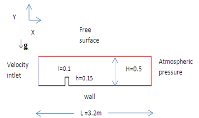 | Figure 1. Geometry and coordinate system |
2.2. Governing Equations
2.2.1. Reynolds Equations for a Monophasic Turbulent Flow
The monophasic turbulent flow in the open-channel flow is described by a set of non-linear partial differential equations expressing the physical laws of conservation between the velocity and pressure at each point of the flow: the Navier-Stokes equations. To these equations, we add the equation of turbulent kinetic energy and that of its dissipation rate like proposed by Launder and Spalding[14]. Solving these equations will reveal features such as pressure, dynamic and void fraction fields. | (1) |
 | (2) |
The relation (1) is a continuity equation, and (2) is the equation of the quantity of movement conservation in which:• the left term represents the convective transport;,• the first term on the right represents the forces due to the pressure;• the second term on the right represents the forces of viscosities;• the two last terms on the right represents the forces generated by the turbulence.The means equations lead to the appearance of the double correlation terms of the velocities fluctuations. They come from the non-linearity of conservation equations. These terms are called Reynolds stress ( ), and translate the effect of turbulence on the evolution of the means movement, giving the equations systems open by introducing supplementary unknowns terms. The closure problem is resolved through the hypothesis of Boussinesq:
 | (3) |
We are going to use for our resolution, the model of turbulence k-ε standard proposed by Fluent which is a model enough used: | (4) |
To determine  , we have to calculate the two variables k and ε. The equations of kinetic energy turbulent and its dissipation rate give us the following relations bellow:For the kinetic energy turbulent
  | (5) |
• the term at the left represent the variation of the kinetic energy turbulent;• the first term at the right represents the production of kinetic energy turbulent;• the second term at the right represents the diffusion;• the last term at the right represents the dissipation.The dissipation energy equation is given by the following relation: | (6) |
Where, Cµ, Cε1 and Cε2 are empirical constants; σε and σk are respectively the turbulent Prandtl numbers relative to k and ε. The values of these constants proposed by Jones and Launder[14], are represented on table 1 bellow. Table 1. Empirical constants proposed by Jones and Launder[14]
 |
| |
|
2.2.2. Reynolds Equations for a Biphasic Turbulent Flow
The numerical resolution of the equation of Navier-stokes incompressible in their non-miscible biphasic Eulerian formulation needs a location of the interface between the different fluids present. The methods based on the capture of the interface, consist to locate the free surface in fix mesh of a means field known in the domain containing the free surface. This method is an opposite approaches used for the interface which consist to follow the deformations of the free surface in the mesh. The major interest of these capture methods is the possibility to simulate flows presenting the interface reconnections. In our present case, the adopted technical is the approach of volume of fluid (VOF), introduced by Hirt and Nichols[16], to solve the topological evolution of a biphasic area. The continuity equation for the phase q is given by the following relations: | (8) |
Where mpq represents the mass transfer of the pth phase at a qth phase: m12 = m21 and mpp = 0. Ρq is the volume mass of the phase q and vq is the volume. The equation of the quantity movement conservation of the phase q is given by the following relation: | (9) |
Where:-  is the shear stress of a qth phase (Pa);-
  is the exterior force of volume (N/kg);-
  is the added mass force (N/kg);-
  is the interaction force at the interface;-
  is the void fraction of phase q.
2.3. Computation Procedure
The transition from physical domain to the numerical domain begins with the generating mesh geometry by a preprocessor. Then import this into a computational code for the iterative solution of equations to determine the values of variables on each node of the mesh. The segregated solution method was chosen for the resolution of turbulence model and governing equations. Governing equations were discredited with the control volume technique. For the convective and the diffusive terms, a second order upwind method was used while the SIMPLE (Semi Implicit Method for Pressure Linked Equations) procedure was introduced for the velocity-pressure coupled to a multiphase model (VOF) (Patankar[17]). The convergence of the numerical calculation is checked by examining the evolution of relative residuals in each governing equation for a convergence criterion of 0.001%. The stability of the iterative process was carried out by relaxation coefficients associated with the velocity, pressure, temperature, κ, ε and μt. The Standard Wall-Functions were used to take into account the effects of friction near the wall. Three mesh distributions have been tested to ensure that the calculated results are grid independent.
3. Results and Discussion
3.1. Generating Mesh Geometry
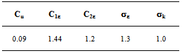
The figure 2 below represents the computational domain meshed with the code GAMBIT. The grid distribution is a set of quadrilateral cells (uniformly structured mesh). The calculations will use the software FLUENT.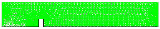 | Figure 2. Grid configuration |
The mesh is very uniformly fine near the obstacle where the velocity gradient is large. The grid distribution impacts the computation time and the number of iterations required for the solution converge. The choice of the mesh size of 16,080 cells is a good compromise and the results that will be presented later are those of this mesh size. The no-dimension variables are: | (10) |
 | (11) |
 | (12) |
 | (13) |
3.2. Pressure Field
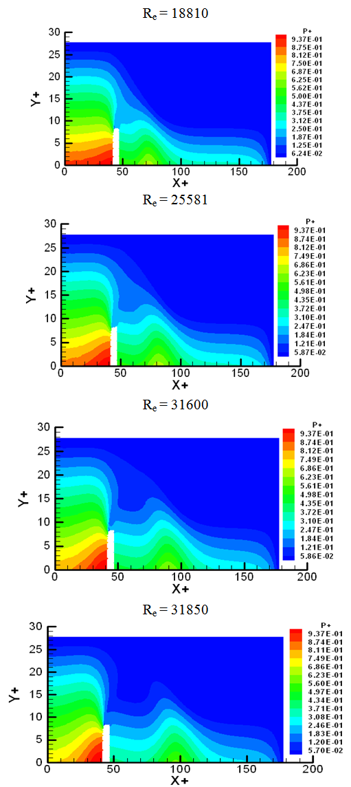 | Figure 3. Pressure field for different Reynolds numbers |
The figure 3 below represents the pressure field for different Reynolds numbers. We observe a pressure loss from the entrance to the outlet generated by fluid friction with the walls and the obstacle. In the upstream from the obstacle region, the fluid comes to dash over the obstacle, and tries to pass around or over. The flow slows down in the downstream from the obstacle generates an inverse pressure gradient. This generates a recirculation flow which creates an oscillatory flow around the obstacle. For the increasing of the Reynolds numbers, the oscillatory flow position goes back to the upstream position. The flow movement is modified after the choc with the obstacle. Near the obstacle, the pressure gradient is very important.
3.3. Dynamic Field
The figure 4 below represents the velocity field for different Reynolds numbers. We observe that the obstacle creates a slow down of fluid particles which are in contact with it. The fluid viscous friction with the obstacle wall generates the velocity decreasing near the obstacle when the Reynolds numbers are increasing. Over the obstacle, we observe a strong accelerated flow because its presence reduces the cross section flow. To compensate this flow reducing near the obstacle wall, the flow is accelerated in the central zone of channel, justifying the mass conservation principle.In the downstream zone near the obstacle, the velocity field is negative and increasing with the Reynolds numbers, showing that a separation of the boundary layer. This is generated by a pressure loss showing a fluid recirculation. The inertia forces are increasing and allowing the boundary layer to remain attached on the obstacle, generating a depression in the wake zone. We observe also an oscillatory flow (vortex), around the obstacle.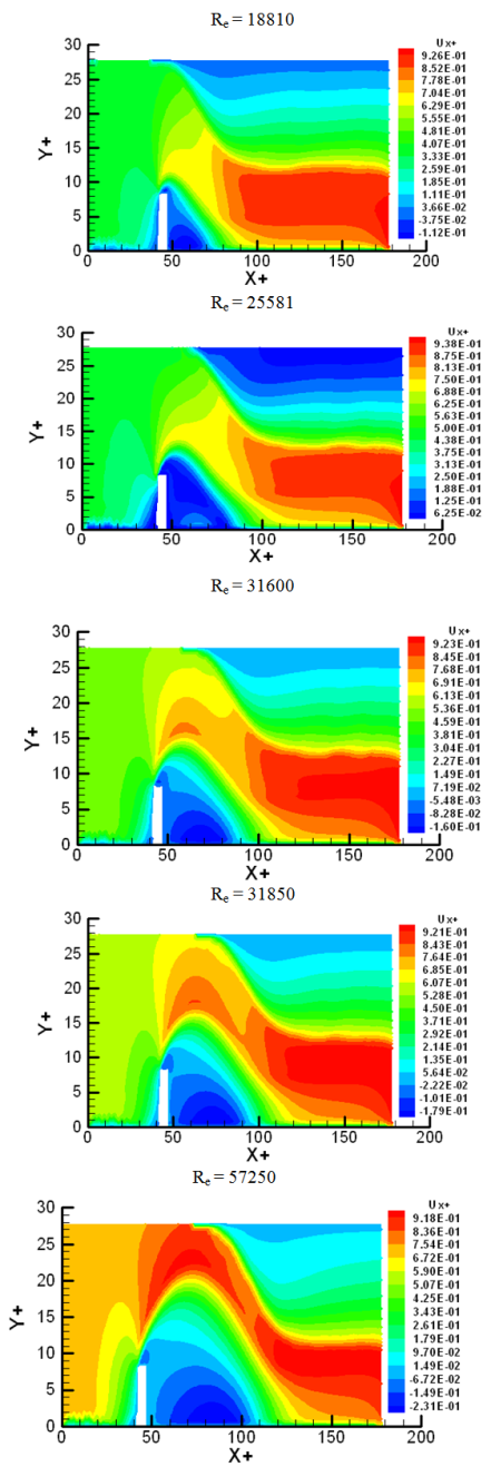 | Figure 4. Longitudinal velocity field for different Reynolds numbers |
3.4. Velocity Profiles Upstream from the Obstacle
The figure 5 below represents the longitudinal velocity profiles in the upstream from the obstacle zone, for two positions of X+ and for different Reynolds numbers. These profiles are not influenced by the obstacle presence, signifying the fully developed flow. The boundary layer thickness decreases with the flow development, until filling the section.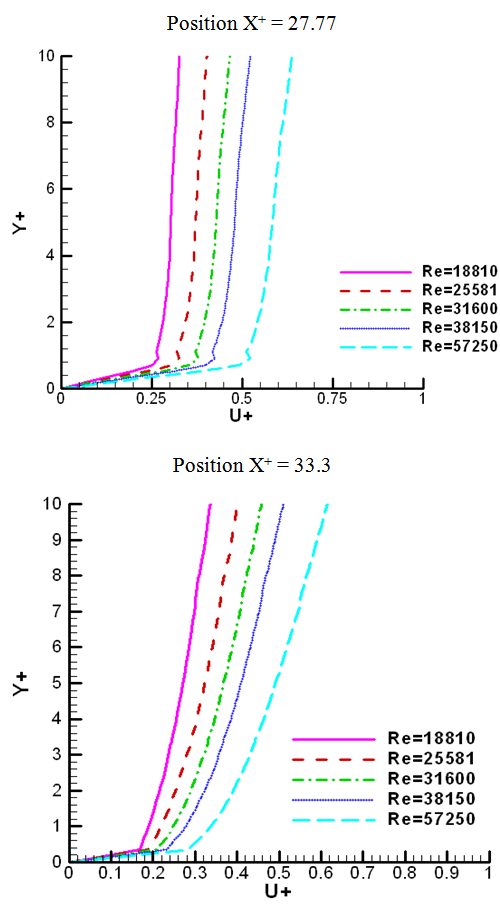 | Figure 5. Longitudinal velocity profiles for different Reynolds numbers in the upstream from the obstacle zone |
3.5. Velocity Profiles Downstream from the Obstacle
The figure 6 below represents the longitudinal velocity profiles at four positions in the downstream from the obstacle zone, for different Reynolds numbers. We observe that the influence of the obstacle on the flow is very important. The velocity decreases in the recirculation flow zone with the increasing of the Reynolds numbers. This velocity decrease continues until it becomes almost zero. The increasing of Reynolds numbers lead to an increase of the recirculation zone height. Above this level, Y+=Y1; we observe a shearing layer generated by the velocity gradients. This extends until the level Y+ = Y2. We suppose that this level is a free surface characteristic, since the velocity is decreasing. The free surface interacts with the flow as an air-package which is closed from above at the higher level of turbulence above the free surface.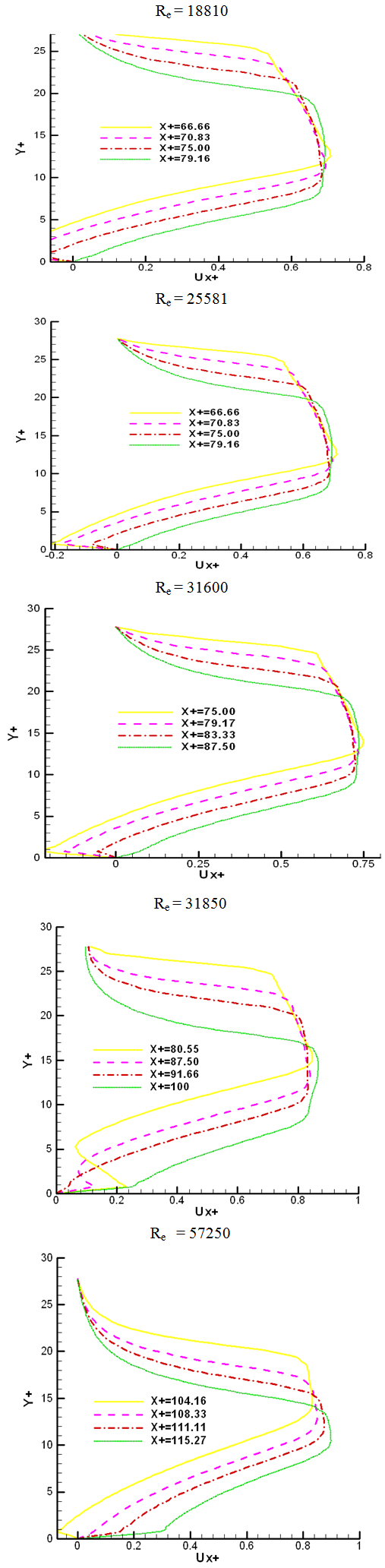 | Figure 6. Longitudinal velocity profiles at four positions in the downstream from the obstacle zone, for different Reynolds numbers |
3.6. Void Fraction Field
The figure 7 below represents the void fraction field for different Reynolds numbers. We observe that the fluctuation level of free surface is increasing with the Reynolds numbers. The presence of air generates the velocity decreasing in the channel flow. This tendency is strong for the highest Reynolds numbers. This could be explained by the friction at the interface air-water which is important when velocity increases. This phenomenon had been related by Tcheukam-Toko and al.[18], in the open-channel flow over the dune. The air-water mixing is generated by the strong interactions between the free surface and the turbulence which generates disturbances of the interface and vortex air-water formation. We have used the VOF method in which interface is determined after the iso-value C= 0.5.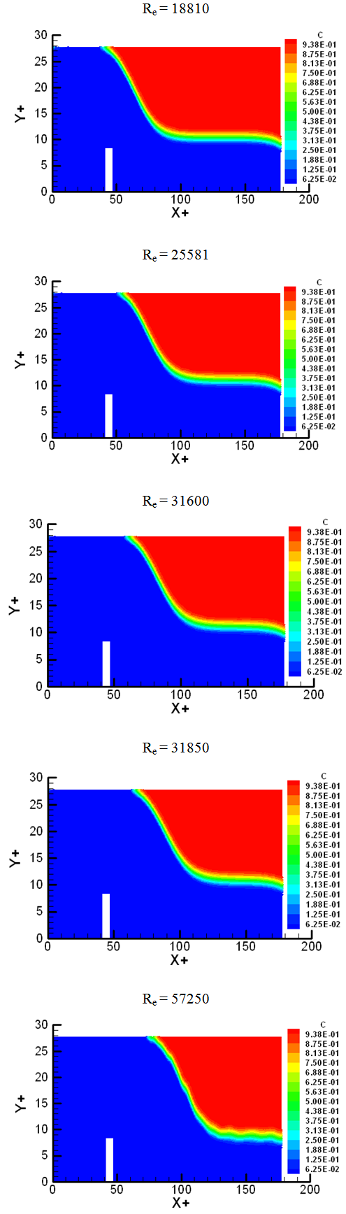 | Figure 7. Void fraction field for different Reynolds numbers |
3.7. Comparison with Experimental Results
The figure 8 below represents the comparison between the void fraction profiles of our numerical results and the experimental results obtained by Murzin and Chanson[10], for different Froude numbers. We observe the distinction in two regions of the vertical void fraction profiles. The first one extends from the bottom of the channel to a well-defined position (y = y*). On this region, the void fraction profiles satisfy a diffusion equation. This was experimentally verified by Chanson and Brattberg[3], Murzin and al.[10].[11],[12]. This region is called, the turbulent sheared layer. Air bubbles were broken up into smaller bubbles and leads into the high shear stress region. The second region extends from y*, up to the free surface. In this part, the air content is strongly dominated by interfacial aeration and large amplitude of the free surface motion. Above the mixing layer, the recirculation and upper flow region was characterized by large air content, splashes and recirculation areas, with large eddies and wavy free surface pattern. Experimentally, Murzin and al.[10],[11],[12], have identified a maximum in the zone of sheared turbulent layer development, while the second maximum is found near the free surface. Our numerical simulation presents also two maximum, but in the sheared layer, the void fraction profile is linear.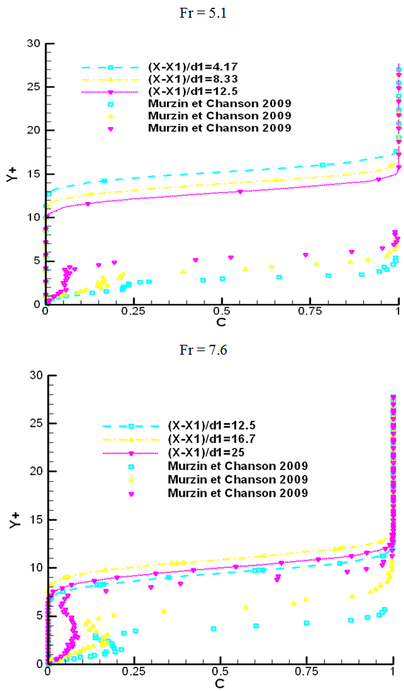 | Figure 8. Comparisons of numerical and experimental void fraction |
The small difference observed between the two results could be explained by these different reasons:• The VOF method is adapted for the capture of the fluids interfaces. It uses distribution function C, which picks up all the flow phases, but without taking into account no mixture, no reaction. It would be interesting to undertake a study with a model based on the Lagrangien approach.Experience was conducted for an hydraulic jump generated by an open gate, while in this present study, the hydraulic jump is generated by a rectangular obstacle.The  model do not take into account the anisotropy effect on the free surface, it would be interesting to use an RSM model or a
  anisotropy.
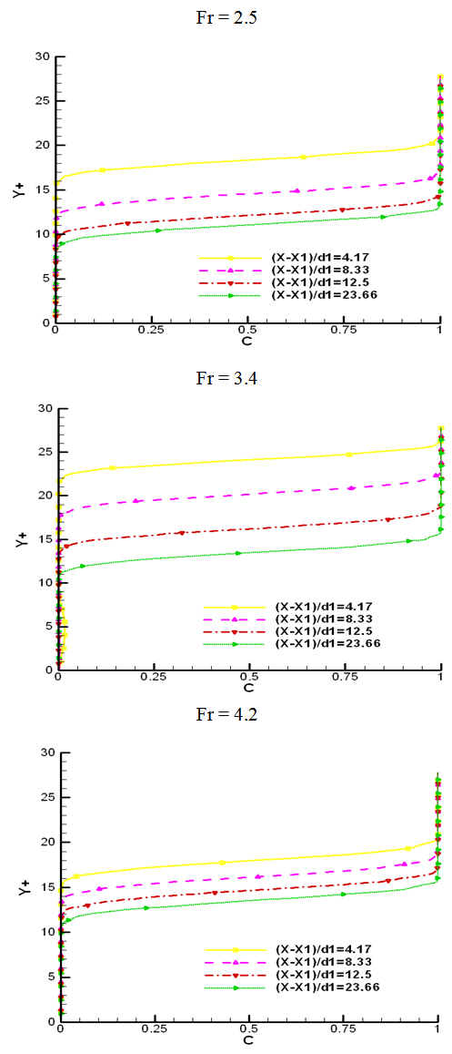 | Figure 9. Numerical void fraction profiles for different Froude numbers |
4. Conclusions
We observe in the pressure field an inversion of pressure gradient which generate the separation of the boundary layer. This is called “back flow phenomenon”. We observe that in the upstream from the obstacle, the velocity is low. At the obstacle level, it appears an acceleration zone with the diminution of the liquid thickness. In downstream from the obstacle, it appears a hydraulic jump where the velocity is very low. The jump behaves as an attractive basin of hydraulic power. If the liquid particles move from the jump towards the upstream where the flow regime is torrential, its propagation velocity is lower than its supercritical flow, and it is brought back towards the jump. In the same manner, if the liquid particles move towards the downstream where the flow regime is fluvial, its propagation velocity is higher than its subcritical flow, and allows it to come back towards the jump. The void fraction profiles are in concordance with the experimental data of Murzin and Chanson.
NOMENCLATURE
C: void fractiond1: hydraulic diameter (m)f: source termD: tube diameter (m)x: axial coordinate (m)y: vertical coordinate (m)L: channel length (m)v: vertical velocity (m/s)u: longitudinal velocity (m/s) : mean of longitudinal velocity (m/s)
 : longitudinal velocity fluctuation (m/s)g: gravitational acceleration (m. s-2)h1; h2: height of hydraulic jump (m)p: pressure (N/m2)Fr: Froude numberRe: Reynolds number = VRh/νGreek symbolsν: kinematic viscosity (m. Kg-1. s-1)ρ: density (kg. m-3)μ: dynamic viscosity (m. Kg-1. s-1)κ: turbulent kinetic energy (m3. s-2)ε: dissipation rate (m3. s-3)φ: wall heat flux (W. m-2)
 : kronecker symbol
 : turbulent viscosity (m2/s)
 : shear stress
References
| [1] | Chanson H. Air entrainment in two dimensional turbulent shear flows with partially developed inflow conditions. International Journal of Multiphase Flow, 1107-1121, 1995. |
| [2] | Mossa M. and Tolve U. Flow visualization in bubbly two-phase hydraulic jump. J. Fluids Eng ASME 120 (March): 160-165, 1998. |
| [3] | Chanson H. Brattberg T. Experimental study of the air-water shear flow in hydraulic jump. International Journal of Multiphase Flow. 495-508, 2000. |
| [4] | Rouse H. Siao T T. Nagaratnam S. Turbulence characteristics of the hydraulic jump. Trans ASCE 124: 926-966. 1959. |
| [5] | Resch F J. Leutheusser H J. Le ressaut hydraulique : Mesure de la turbulence dans la région diphasique. La Houille Blanche, 279-293, 1972. |
| [6] | Resch F J. Leutheusser H J. Reynolds stress measurements in hydraulic jump. J Hydraulic Research IAHR 10(4): 409-429, 1972. |
| [7] | Chanson H., Air bubble entrainment in free surface turbulent shear flow. Academy Press, London 401 P, 1997. |
| [8] | Liu M. Rajaratnam N. Zhu D. Turbulence structure of hydraulic jumps of low Froude number.J.Hydraulic Eng. 130(6): 511-520. 2004. |
| [9] | Mouaze D., Murzyn F and Chaplin J R. Free surface length scale estimation in hydraulic jumps.Journal of Fluids Eng., 1191-1193,2005. |
| [10] | Murzyn F. Chanson H. Experimental investigation of bubbly flow and turbulence in hydraulic jumps. Environmental Fluid Mechanic, pp. 143-159. 2009. |
| [11] | Murzyn F. Chanson H. Free surface fluctuations in hydraulic jumps: Experimental observations. Experimental Thermal and Fluid Mechanic. pp. 1055-1064. 2009. |
| [12] | Murzyn F. Chanson H. Two phase flow measurements in turbulent hydraulic jumps. Chemical Engineering Research and Design. 789-797, 2009. |
| [13] | Vigie Franc. Etude expérimentale d’un écoulement à surface libre au-dessus d’un obstacle. Thèse de Doctorat de l’Institut National Polytechnique de Toulouse. 175 p, 12 octobre 2005. |
| [14] | Launder, B., E., Spalding, D. The numerical computation of turbulent flows computational methods. App. Mech. Engineering, Vol. 3, pp. 269-289. 1974. |
| [15] | Fluent 6.3.26 User manual 2006. |
| [16] | Hirt C W. Nichols B D. Volume of fluid (VOF) methods for the dynamics of free boundaries. J. Comp. Phys. 39, pp. 201-225. 1981. |
| [17] | Patankar S.V., 1980. Numerical heat transfer and fluid flow, McGraw Hill, New-York. |
| [18] | Tcheukam-Toko D.,Movahedam M. Berlogey M. Study of turbulent friction in a gradually varied flow. Research Journal and Applied Sciences. pp. 465-470. 2008. |
 Abstract
 Reference
 Full-Text PDF
 Full-text HTML